Each toolbar contains a group of icon buttons that provide access to common
tools.
Toolbars are dockable, meaning they can be moved and either floated or pinned to a
location, allowing you to configure the workspace according to your preferences.
Turn toolbars on and off from the menu bar by clicking View > Toolbars.
Checks
The Checks toolbar provides access to checks and calculations tools that are commonly
used in the model building process.
Turn the Checks toolbar on and off
from the View > Toolbars > Checks menu. Figure 1.
Left-click: Reverses the mask state of all elements in currently
displayed collectors.
Right-click: Reverses the mask state of all entities (elements, loads,
and so on) in currently displayed collectors.
Unmasks the row of elements adjacent to the currently displayed ones. If
some of the unmasked elements reside in components that are currently
not displayed, those components will also be unmasked.
Unmasks all entities (elements, loads, and so on) in the currently
displayed collectors.
Left-click: Masks all entities (elements, loads, and so on) located
outside of the graphics area but in currently displayed collectors.
Right-click: Unmask all entities (elements, loads, and so on) located
outside of the graphics area but in currently displayed collectors.
Displays a scale in the lower, right-hand corner of the graphics area,
which you can use to measure different parts of your model. The numbers
on the scale are dependent upon the dimension of the model and the zoom
factor you are currently using in the graphics area.
Switches the display of element handles on/off.
Switches the display of load handles on/off.
Points the load vector toward the load application point (tip), or away
from the load application point (tail) when the tip or the tail of the
load vector is attached to the load application point.
Note: The
direction of the vector does not change when you select this
option.
Switches the display of fixed points on/off.
Favorites
The Favorites toolbar allows you to save and access a menu that lists your favorite
panels. HyperMesh saves the list of favorite panels and
restores it accordingly when you start a new session.
Turn the Favorites toolbar on and
off from the View > Toolbars > Favorites menu. Figure 4.
Patch Checker
The Patch Checker toolbar contains a group of icon buttons that you can use to review
quality results, sliver surfaces, elements attached to selected nodes, and so
on.
Entities placed on the user mark are used as input. The user mark is populated by
selecting the save option from advanced entity selections,
specific panels that have the save button (such as Check Elems), or via Tcl script
using *marktousermark.
This tool creates "patches", or local regions, from each input entity. A patch
includes only displayed entities. Patches are not created for any input entities
that are not displayed. A spherical clipping is then calculated and applied for each
patch, with the input entity highlighted and the adjacent entities low lighted. In
order to keep the performance high, only the first 500 entities on the user mark are
considered.
Turn the Patch Checker toolbar on
and off from the View > Toolbars > Patch Checker menu. Figure 5.
Select the elements entity type.
Select the surfaces entity type.
Select the nodes entity type.
Turn the tool on or off.
Go to the previous patch.
Go to the next patch.
Go back to the first patch.
Decrease the size of the spherical clip.
Increase the size of the spherical clip.
Reset the spherical clip back to its default.
Undo-Redo
The Undo-Redo toolbar provides access undo and redo functionality.
Turn the Undo-Redo toolbar on and
off from the View > Toolbars > Undo-Redo menu. Figure 6.
Visualization
The Visualization toolbar contains a group of icons that you can use to control the
display of entities in the graphics area.
Turn the Visualization toolbar on
and off from the View > Toolbars > Visualization menu. Figure 7.
Geometry - Color mode options
Automatically select a color mode based on the active
panel.
You can change display colors in the Options panel, Colors
subpanel.
All surfaces are colored based on the assemblies they belong
to. Each assembly receives a different color (although
models with many assemblies may have colors repeated for
more than one assembly). Any surfaces that do not belong to
an assembly are colored gray.
All surfaces are colored based on the parts they belong to.
Any surfaces that do not belong to a part receive the color
assigned to the main model.
Changes the color of all surfaces and solid faces to the
color assigned to the component in which that geometry
resides. All surface edges and solid face edges are colored
black.
Surfaces are colored gray (2D faces (topo) with surface
edges colored by topology: red (free edges), green (shared
edges), yellow (t-junctions), or blue (suppressed edges).
Solid faces and face edges are colored transparent green
(bounding faces) with internal faces colored yellow (full
partition faces).
Surfaces are colored gray (2D faces (topo) with surface
edges colored by topology: red (free edges), green (shared
edges), yellow (t-junctions), or blue (suppressed edges).
Solid faces and face edges are colored blue, ignoring solid
topology.
Surfaces and surface edges are colored blue, ignoring
surface topology. Solid faces and face edges are colored
transparent green (bounding faces) with internal faces
colored yellow (full partition faces).
Surfaces are colored by component with surface edges colored
by topology. Solid faces are colored by component with solid
face edges colored by topology.
Surfaces display in wireframe mode, with surface edges
colored blue (ignoring topology). Solid faces are colored by
mappability: red (not mappable), yellow (1d mappable), or
green (3d mappable). Solid face edges are colored by
topology.
Geometry - Shade options
Set geometry mode to shaded with surface edges.
Set geometry mode to shaded.
Geometry - Wireframe options
Set geometry to wireframe with surface lines.
Set geometry to wireframe mode.
Opens the Transparency panel.
Mesh - Color mode options
All elements are colored based on the parts they belong to.
Any elements that do not belong to a Part receive the color
assigned to the main model.
All elements are colored by the color assigned to the
component in which that element resides.
All elements are colored by the property assigned to that
element. Properties are assigned to elements directly or
indirectly. Properties are assigned directly to the element
by using the Property > Assign panel. Indirect element
properties are inherited from the component in which the
element resides; component properties are assigned in the
Component > Assign panel. Directly assigned properties
override indirect ones. Solvers in group #1 (Radioss (Bulk Data), OptiStruct, Nastran) can support both direct and
indirect element property assignment. Solvers in group #2
(Radioss (Block), LS-DYNA) only support indirect element
property assignments. Any element without a property is
colored gray.
All elements are colored by the material assigned to that
element. Materials are assigned to elements differently for
solver group #1 and solver group #2; Solver Group #1
(Radioss (Bulk Data),
OptiStruct, Nastran) assign materials to
properties, and then properties to elements (either directly
or indirectly as discussed in Color by Property). Elements
with both direct and indirect property assignments use the
material associated with the direct element property
assignment. Solver group #2 (Radioss (Block), LS-DYNA) assigns materials to elements
indirect by assigning materials to the component in which
the element resides using the Component > Assign panel. Any
element which does not have a material assigned to it,
directly or indirectly, will be colored gray.
All elements are colored based on the assemblies they belong
to. Each assembly receives a different color (although
models with many assemblies may have colors repeated for
more than one assembly). Any elements that do not belong to
an assembly are colored gray.
All elements are colored by their topology: green (1D), blue
(2D), and red (3D).
All elements are colored by their element configuration
(mass, reb2, spring, bar, rod, gap tria3, quad4, tetra4, and
so on).
Opens the Thickness
View, and colors shell elements according to
their thickness values. Both element as well as node
thicknesses are supported. A thickness legend is shown in
the upper-left corner of the graphics area.
Thickness coloring can be combined with 2D Detailed Element
Representation Figure 8. Element Thickness with 2D Detailed
Representation Figure 9. Nodal Thickness with 2D Detailed
Representation
This permanent mode serves as a useful tool to investigate
each specific element criteria, as well as evaluate the
overall quality of a mesh.
All elements are colored based on the domains they belong
to. A domain is a morphing entity which enables design
changes to an existing FE topology. Each domain receives a
different color. Any elements that do not belong to a domain
are colored gray.
Elements - Shaded options
Set current element visual mode to shaded with mesh lines.
Elements are shaded, and surface mesh lines display.
Set current element visual mode to shaded with feature
lines. Elements are shaded but have no mesh lines, while
feature lines display.
Set current element visual mode to shaded. Elements are
shaded, but no lines display.
Elements - Wireframe options
Set the current element visual mode to wireframe (skin
only). Internal mesh lines will not display.
Set the current element visual mode to wireframe. Internal
and surface mesh lines display.
Set current element visual mode to transparent
with elements and feature lines. Elements
are shaded but transparent, no mesh lines display, but
feature lines do.
1D - Element options
Display a more detailed, shaped-based representation for 1D
beam elements.
Display both the simple and detailed representations for 1D
beam elements.
2D - Element options
Display a simple representation for 2D shell elements.
Display a more detailed, shaped-based representation for 2D
shell elements.
Display both the simple and detailed representations for 2D
shell elements.
Ply/Composite options
Ply layers are not displayed.Figure 10.
Plies in a composite material are displayed. Figure 11.
The exact nature of the display depends on the 2D
Element Representation button. See Element and Ply Visualization for
details.
For continuum shells the display can be overlaid with the
transparent representation of the original continuum shell
elements, if 2D Traditional Element
Representation () is turned on.
Display layers with vectors indicating their appropriate ply
orientation. Corrected fiber directions are shown if the
drape data is available on every element of the ply.Figure 12.
The exact nature of the display depends on the 2D/3D
element visualization button. See Element and Ply Visualization for
details.
For continuum shells the display can be overlaid with the
transparent representation of the original continuum shell
elements, if 2D Traditional Element Representation () is turned on.
Enables the ply lay-up or stack boundaries to be visualized,
which provides an easy way to view ply drop-off. When the
stack topology shape is changed, the visualization of the
edges is automatically updated. Ply layer geometry edges are
always outlined in white, where as FE edges are always
outlined in the same color as the ply. FE edges are always
outlined with a thicker line compared to geometry
edges.
Toggle on/off shrink elements by shrink factor.
Shrink factor can be set from the Options panel, Graphics subpanel.
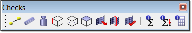


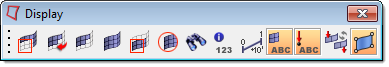


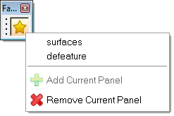
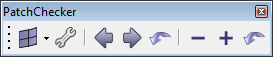


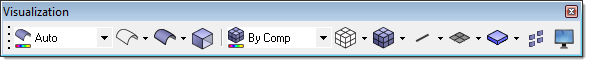


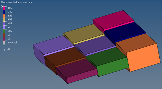
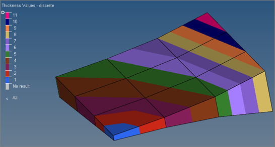


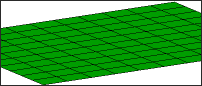

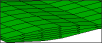 Figure 11.
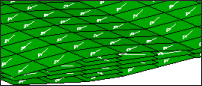 Figure 12.

