Exercise 2: Define Boundary Conditions and Loads for the Seat Impact Analysis
In this exercise, you will define boundary conditions and load data for an LS-DYNA analysis of a vehicle seat impacting a rigid block.
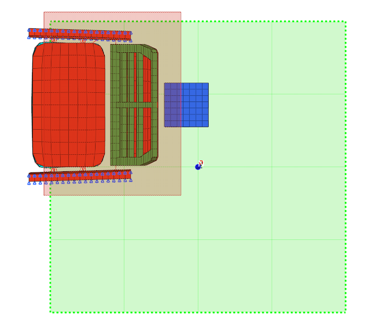
Figure 1.
Load the LS-DYNA User Profile
In this step, you will load the LS-DYNA user profile in Engineering Solutions.
- Start Engineering Solutions Desktop.
- In the User Profile dialog, set the user profile to LsDyna.
Retrieve the Engineering Solutions File
In this step, you will open the model file in Engineering Solutions.
-
Open the model file by completing one of the following options:
- Click from the menu bar.
- Click
 on the Standard toolbar.
Define Gravity Acting in the Negative Z-Direction
In this step, you will define gravity acting in the negative z-direction with *LOAD_BODY_Z.
-
In the Solver Browser, right-click and select from the context menu.
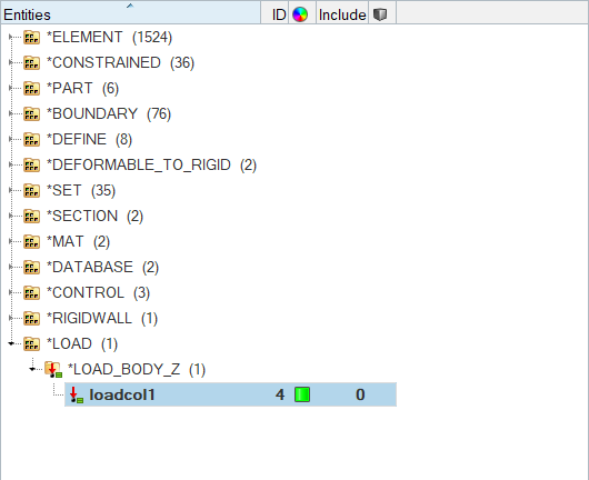
Figure 2.Engineering Solutions creates and opens a new load collector in the Entity Editor. -
Click LCID, and then click
curve.
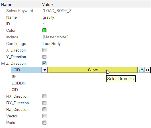
Figure 3.The Select Curve dialog opens. -
In the Select Curve dialog, select gravity
curve and then click OK.
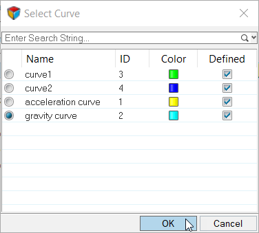
Figure 4.
Define the Seat Acceleration
In this step, you will define the seat acceleration with *BOUNDARY_PRESCRIBED_MOTION_NODE.
-
Create a load collector.
-
In the Model Browser, right-click and select from the context menu.
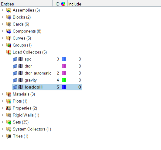
Figure 5.Engineering Solutions creates and opens a new load collector in the Entity Editor.
-
In the Model Browser, right-click and select from the context menu.
-
Create acceleration loads on nodes.
Export the Model
In this step, you will export the model to an LS-DYNA 971 formatted input file.
- From the menu bar, click .
- In the Export - Solver Deck tab, set File type to Ls-Dyna.
- In the File field, navigate to your working directory and save the file as seat_complete.key.
- Click Export.
Submit the Input File
In this step, you will submit the LS-DYNA Input File to LS-DYNA 971.
- From the Start Menu on your desktop, open the LS-DYNA Manager program.
- From the solvers menu, select Start LS-DYNA analysis.
- Load the seat_complete.key file.
- Click OK to start the analysis.
View the Results in HyperView
In this step, you will view the results in HyperView.
Save your work as a Engineering Solutions file.