3D Shooting and Bouncing Rays
The Shooting and Bouncing Rays (SBR) method performs a rigorous 3D ray-launching prediction which results in a high accuracy, but it can be computationally expensive.
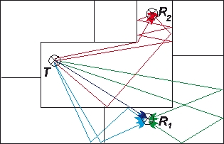
Figure 1. Principle of ray optical models.
As smaller wavelengths (higher frequencies) are considered, the wave propagation becomes similar to the propagation of light. Therefore a radio ray is assumed to propagate along a straight line influenced only by refraction, reflection, diffraction or scattering which is the concept of geometrical optics (GO). The criterion taken into account for this modeling approach is that the wavelength should be much smaller than the extension of the considered obstacles, for example, the walls of a building. At the frequencies used for mobile communication networks this criterion is also inside buildings sufficiently fulfilled.
- ray-tracing
- ray launching
Propagation Paths
Each transmission through a wall, each reflection at a wall and each diffraction at an edge counts as an interaction. The computed propagation paths can be limited within the propagation model settings. The value Max. defines the maximum number of interactions that are allowed for each propagation path. The appropriate value depends on the building structure. If, for example, the building has a corridor that runs around a corner three times, then it would be better to compute more interactions, because multiple diffractions are needed to reach all prediction pixels. The same occurs if a building has a structure where the rays have to pass many walls to reach every point of the building, because then more transmissions are needed. The only constraint is that the computation time naturally increases if more interactions are computed. On the other hand, if too few interactions are computed, the accuracy decreases. In this case additionally more prediction pixels might not be reached by the SBR prediction, which leads to the need to compute those pixels with an empirical model which will decrease the accuracy even more. As a basic rule, an appropriate setting for the maximum value would be 2 – 4, depending on the building structure.
Computation of Each Ray's Contribution
The deterministic model uses Fresnel equations for the determination of the reflection and transmission loss and the GTD / UTD for the determination of the diffraction loss. This model has a slightly longer computation time and uses three physical material parameters (permittivity, permeability and conductivity). When using GTD / UTD and Fresnel coefficients arbitrary linear polarizations (between +90° and –90°) can be considered for the transmitters.
The effect of bookshelves and cupboards covering considerable parts of walls is taken into account by including an additional loss of the wall's penetration (transmission) loss. An additional loss of 3 dB was observed to be appropriate. This additional loss is introduced in context of walls covered by bookshelves, cupboards or other large pieces of furniture. Furthermore, it was found necessary to set an empirical limit for the wall transmission loss which otherwise becomes very high when the angle of incidence is large.
- Specular Reflection
-
The specular reflection phenomenon is the mechanism by which a ray is reflected at an angle equal to the incidence angle. The reflected wave fields are related to the incident wave fields through a reflection coefficient which is a matrix when the full polarimetric description of the wave field is taken into account.
The most common expression for the reflection is the Fresnel reflection coefficient which is valid for an infinite boundary between two media, for example, air and concrete. The Fresnel reflection coefficient depends on the incident wave field and upon the permittivity and conductivity of each medium. The application of the Fresnel reflection coefficient formulas is very popular and these equations are also applied in ProMan.
To calibrate the prediction model with measurements, some ray optical software tools consider an empirical reflection coefficient varying with the incidence angle to simplify the calculations. Such an empirical approach is also available in ProMan.
- Diffraction
-
The diffraction process in ray theory is the propagation phenomena which explain the transition from the lit region to the shadow regions behind the corner or over the rooftops. Diffraction by a single wedge can be solved in various ways: empirical formulas, perfectly absorbing wedge, geometrical theory of diffraction (GTD) or uniform theory of diffraction (UTD).
The advantages and disadvantages of using either one formulation is difficult to address since it may not be independent on the environments under investigation. Indeed, reasonable results are possible with each formulation. The various expressions differ mainly from the approximations being made on the surface boundaries of the wedge considered. One major difficulty is to express and use the proper boundaries in the derivation of the diffraction formulas. Another problem is the existence of wedges in real environments: the complexity of a real building corner or of the building’s roof illustrates the modeling difficulties.
Despite these difficulties, however, diffraction around a corner or over rooftop are commonly modeled using the heuristic UTD formulas since they are well behaved in the lit/shadow transition region, and account for the polarization as well as for the wedge material. Therefore these formulas are also used in ProMan to calculate the diffraction coefficient.
- Multiple Diffraction
-
For the case of multiple diffraction the complexity increases dramatically. One method frequently applied to multiple diffraction problems is the UTD. The main problem with straightforward applications of the UTD is that in many cases one edge is in the transition zones of the previous edges. Strictly speaking this forbids the application of ray techniques, but in the spirit of the UTD the principle of local illumination of an edge should be valid. At least within some approximate degrees, a solution can be obtained which is quite accurate in most cases of practical interest.
The key point in the theory is to include slope diffraction, which is usually neglected as a higher order term in an asymptotic expansion, but in the transition zone diffraction the term is of the same order as the ordinary amplitude diffraction terms. Additionally there is an empirical diffraction model available which can easily be calibrated with measurements.
- Scattering
-
Rough surfaces and finite surfaces (surfaces with small extension in comparison to the wavelength) scatter the incident energy in all directions with a radiation diagram that depends on the roughness and size of the surface or volume. The dispersion of energy through scattering means a decrease of the energy reflected in specular direction.
This simple view leads to account for the scattering process by only decreasing the reflection coefficient. The reflection coefficient is decreased by multiplying it with a factor smaller than one where this factor is exponentially dependent on the standard deviation of the surface roughness according to the Rayleigh theory. This description does not take into account the true dispersion of radio energy in various directions, but accounts for the reduction of energy in the specular direction due to the diffuse components scattered in all other directions.
- Penetration and absorption
- Penetration loss due to building walls have been investigated and found
to be dependent on the particular system. Absorption due to trees or the
body absorption are also propagation mechanisms difficult to quantify
with precision. Therefore in the radio network planning process adequate
margins should be considered to ensure overall coverage. Another
absorption mechanism is the one due to atmospheric effects. These
effects are usually neglected in propagation models for mobile
communication applications at radio frequencies but are important when
higher frequencies (for example 60 GHz) are used.
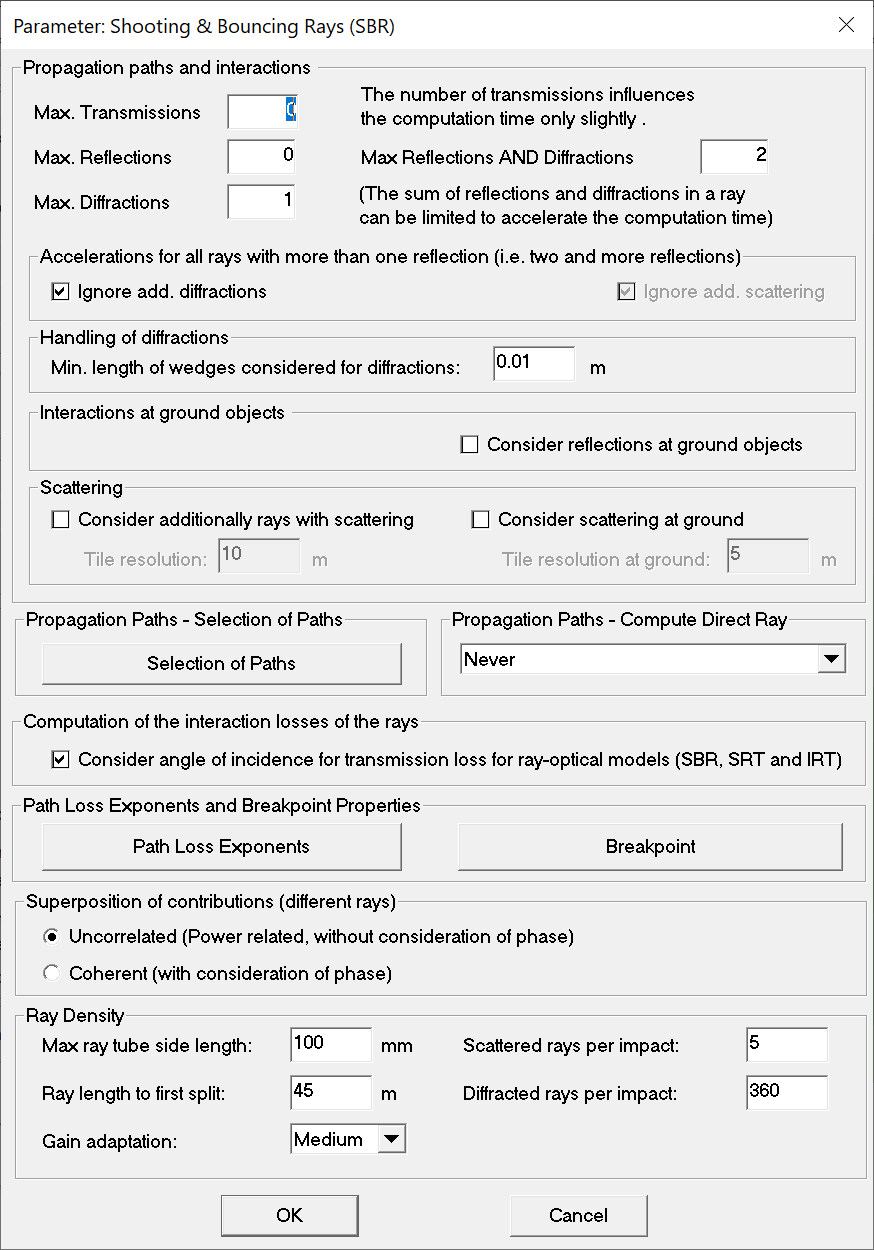
Figure 2. The Parameter: Shooting & Bouncing Rays (SBR) dialog. - Propagation Paths and Interactions
-
The Propagation paths and interactions group allows to specify the number of interactions that should be considered for the determination of ray paths between transmitter and receiver including the maximum number of reflections, diffractions and scattering. To accelerate the prediction, additional diffractions and transmissions can be ignored for all rays with more than one reflection. The minimum length of wedges where diffractions can occur can be specified in meters. In case the simulation database contains ground objects (topography in vector format), interaction at those objects can optionally be considered. Diffuse scattering in indoor scenarios can play an important role, especially for determining the actual temporal and angular dispersion of the radio channel.
The WinProp SBR model was extended to consider the scattering on building walls and other objects. For this purpose the scattering can be activated in the model settings by enabling the option “Consider additionally rays with scattering”. As the scattering increases the overall number of rays significantly, there is a limitation of one scattering per ray. Furthermore, the surface roughnesses of the corresponding materials need to be defined (in WallMan and / or ProMan).
For the scattering in the SRT model, tiles as defined in the dialog are considered. The scattered contribution is weighted with the size of the scattering area (tile). Accordingly the resulting scattered power from the whole object is for large distances independent of the tile size. For small distances there is an impact due to the modified scattering angles which depend on the tile size.
- Propagation Paths - Selection of Paths
-
This option allows the limitation of the number of paths per pixel with the following options: maximum path loss of rays, maximum number of paths or dynamic range of paths.
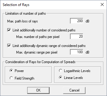
Figure 3. The Selection of Rays dialog.Tip: The computation time of SBR can be reduced significantly by reducing the Max. path loss of rays. Rays that encounter too much path loss will already be discarded during the computation.Note: To accelerate the computation, SBR will estimate the path loss of a ray based on empirical loss parameters. This way, rays which certainly are insignificant can be rejected early. The final signal level of a ray will still be predicted using the user-specified mode (based on Empirical Losses or on Fresnel Coefficients and GTD/UTD). - Propagation Paths - Direct Ray
- The direct ray can be computed always, despite the number of transmissions specified in the first section.
- Computation of interaction losses of the rays
-
For the computation of the rays, not only the free space loss has to be considered but also the loss due to the transmissions, reflections and (multiple) diffraction. This is either done using a physical deterministic model or using an empirical model similar to the method for the intelligent ray-tracing (IRT). Optionally the interaction losses of the rays can be determined considering the angle of incidence for the calculation of the transmission loss.
- Path Loss Exponent for ray-optical models
- Exponent for distance-dependent path loss.
- Ray density
-
Since the SBR method starts by launching rays from the antenna, and, contrary to SRT, doesn’t guarantee that every possible path will be found, the ray density parameters are important.
The Max ray tube size length determines the minimum geometrical detail size that will affect the rays. As the outgoing ray tubes expand, they will be split to ensure that any ray tube cross section does not become too large.
The Ray length to first split is the distance at which the splitting will commence. This length, in combination with the maximum tube size, determines the number of rays that will be launched. For instance, if this length is 1 m and the maximum tube size is 10 cm, then 1257 rays will be launched to cover the 1-meter sphere with area 4π m2. The split rays travel on and multiply as needed.Tip: Ray length to first split is ideally set such that it is at least the distance between the transmitter and the closest geometry. If the distance is set too small, unnecessary splits need to be computed. If the distance is set too large, the ray density close to the transmitter becomes unnecessarily high. The distance to first split will be reduced if needed to ensure that no more than 50 million rays be launched from the transmitter.The Gain adaptation determines to what extend a higher ray density will be used in directions with higher antenna gain. Options are Off, Low, Medium, High.- Low
- If the antenna gain for a direction is higher than MaxGain - 1 * 6dB the density will be increased for that direction by a factor of 2 (side length).
- Medium
-
If the antenna gain for a direction is higher than MaxGain - 2 * 6dB the density will be increased for that direction by a factor of 2 (side length).
If the antenna gain for a direction is higher than MaxGain - 1 * 6dB the density will be increased for that direction by a factor of 4 (side length).
- High
-
If the antenna gain for a direction is higher than MaxGain - 3 * 6dB the density will be increased for that direction by a factor of 2 (side length).
If the antenna gain for a direction is higher than MaxGain - 2 * 6dB the density will be increased for that direction by a factor of 4 (side length).
If the antenna gain for a direction is higher than MaxGain - 1 * 6dB the density will be increased for that direction by a factor of 8 (side length).
Scattered rays per impact determines how many new rays are spawned at each scattering interaction. If the physics of the scattering predicts a lobe in a certain direction, then the density of new rays in that lobe will automatically be higher than in other directions.
Diffracted rays per impact determines how many new rays are created at each diffraction interaction.