Using Multipole in newFASANT to Compute Mutual Coupling in Near-Field

A training example to compute the array coupling in Near-Field using multipoles and GTD module in newFASANT is presented.

The first step is to calculate the multipole using the MoM module and export it to be used to compute the array coupling in Near-Field. You can find it on the next link:

• Multipole Array Simulation

In order to generate the multipole file, an array close to a sphere is created and it will be used as the passive antenna in this training example.

Note that in version 6.3 only is able to compute the coupling with only one element of the passive array. In new improvements, a more general formulation for the coupling between arrays will be stated. We explode all the array elements except this one selected for coupling calculation in order to get only one antenna in the array (other elements will be considered as passive scatters).

In this case, the exploded array elements are grouped and the simulation is selected as shown.

The size of the multipole is set up to 2*wavelengths, therefore the multipole can be used accurately for distances greater than 2*((2*0.1)**2)/0.1=0.8 m.

Then, the simulation is meshed, calculated and saved the multipole generated.

More information about how to do a multipole simulation and how to export this file are in the next links:

• Multipole Simulation
• Export Multipole File

Once the multipole has been created, the GTD project can be started.

Step 1: Create a new GTD Project.

Open newFASANT and select 'File' --> 'New' option.

Select 'GTD' option on the previous figure and start to set up the project.

Step 2: Create the geometry model. To obtain more information about geometries generation see Geometry Menu.

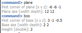
Execute 'plane' command writing it on the command line and set up the parameters as the next figure shown when the command line asks for it.

Execute 'box' command writing it on the command line and set up the parameters as the next figure shown when the command line asks for it.

Step 3: Set up Simulation Parameters.

Select 'Simulation' --> Parameters option on the menu bar and the following panel appears. Set up the parameters as the next figure shows and save it.

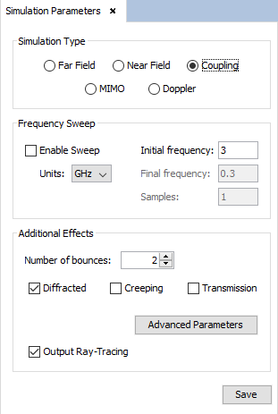
Note: It is important to select ‘Output Ray-Tracing’ to be able to visualize the ray-tracing.

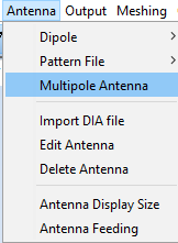
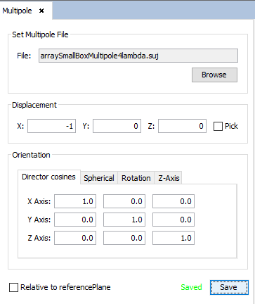
Step 4: Set up the active antenna.

Select ‘Antenna’ --> ‘Multipole Antenna’ and select the arraySmallBoxMultipole4lambda.suj file and locate the antenna at (-1.0, 0.0, 0.0).

Note the file arraySmallBoxMultipole4lambda.suj is the multipole file obtained in the Multipole Array Simulation.

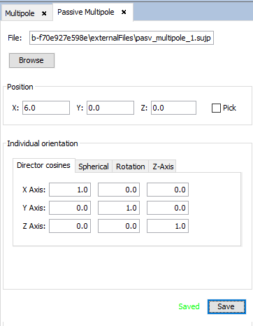
Step 5: In the output menu, the multipole option is selected, input the multipole of the array near sphere of the previous example (only one element is active). Select the array2oneDipole.suj file and locate it at (6.0, 0.0, 0.0).

Step 6: Meshing the geometry model.

Select 'Meshing --> 'Create visibility matrix' and select the number of processors.

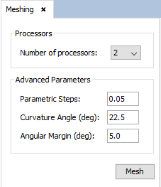
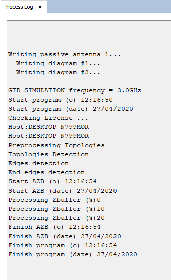
Then click on 'Mesh' button to starting the meshing. A panel appears to display meshing process information.

Step 7: Execute the simulation.

Select 'Calculate --> 'Execute' and introduce the number of processors to be used.

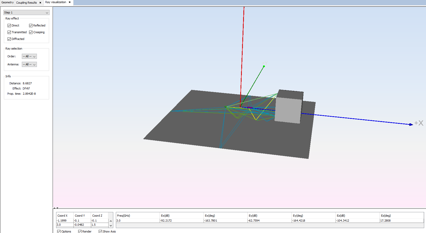
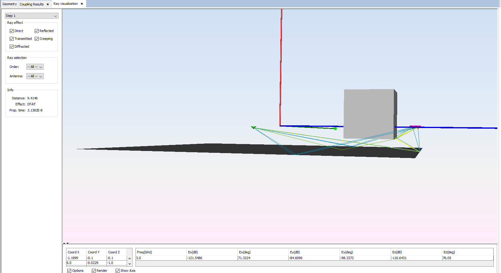
Step 8: After obtaining the results, choose view ray from show results. It is possible to visualize the order 1 ray. It is possible to represent the ray-tracing interacting with the geometry.

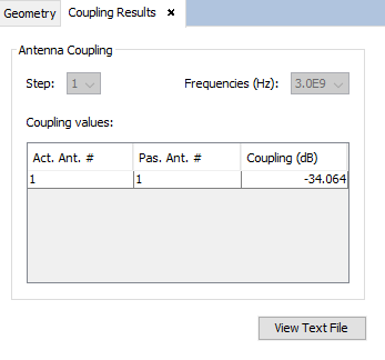
Step 9: Coupling.

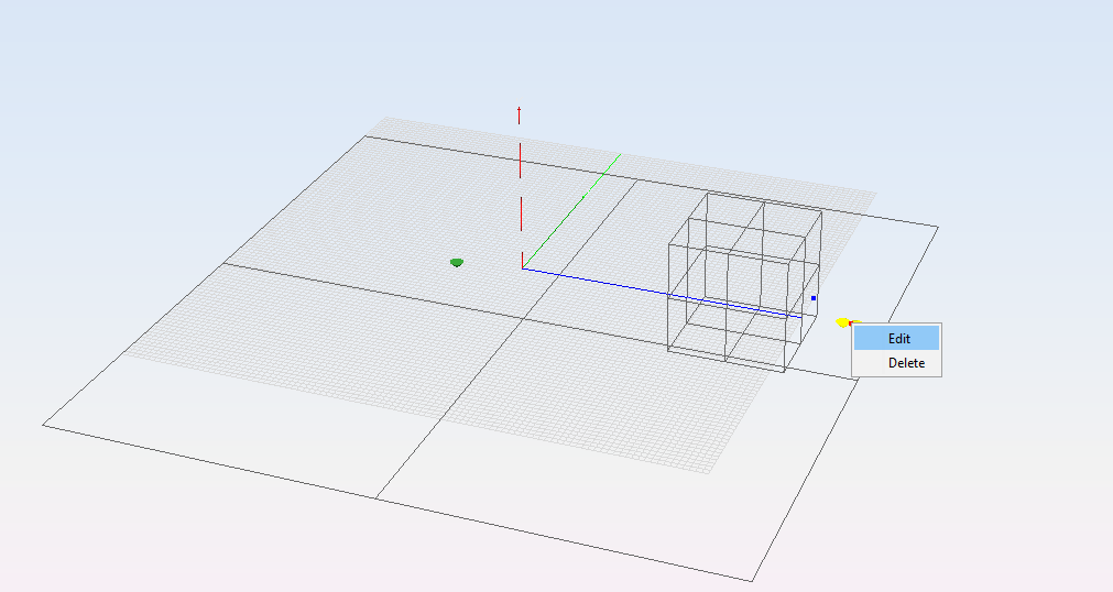
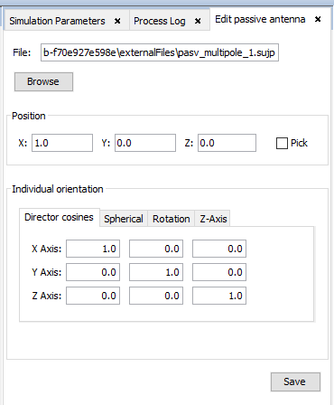
Step 10: In order to modify the location of the passive multipole, the user has to click on the cones with the right button of the mouse, and then the click on ‘Edit’, as is shown in the next figure.

Step 11: Now, the passive multipole is located at (1.0, 0.0, 0.0).

Step 12: A new coupling value and a new ray-tracing between the active array and the dipole in the passive array are obtained.