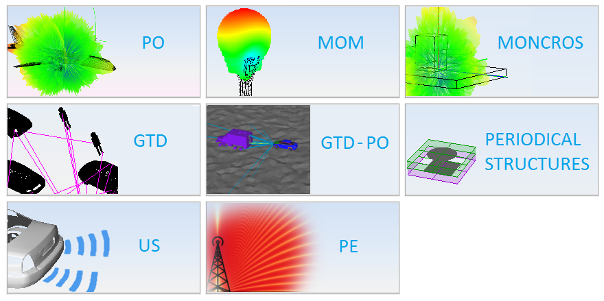
In this section a simple example of a Far Field simulation will be shown. This
simulation will be performed considering a cube as the geometry. An antenna will be
configured to feed this geometry.
Step 1. The first step consists of creating a new data file where all the
parameters of the simulation will be saved. Use the command ‘New’ from the File
menu. Select GTD type.
Figure 1. Selection Method dialog box
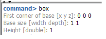
Step 2. The second step is to generate the box. Select Geometry→ Solid → Box.
It will be located at (0,0,0) and the dimensions are 1x1x1 m.
Figure 2. Create box
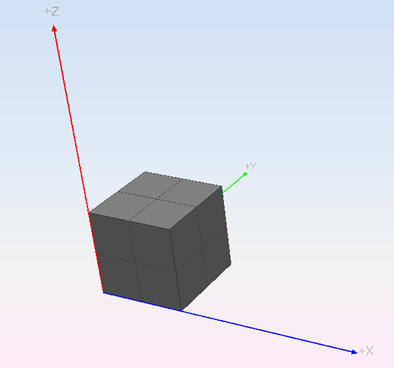
Figure 3. Box situated at (0,0,0)
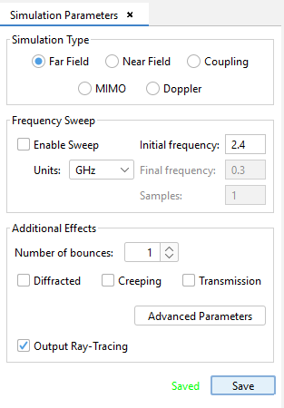
Step 3. The next step is to set the main parameters of the simulations, which
are located in Simulation Parameters Menu → Simulation.
A dialog appears. In this menu, the frequency, number of antennas, kind of
simulation, effects to calculate, and other parameters must be defined before
running the simulation. In this example, a radiation pattern file in far field is
simulated. The user will introduce:
Far field in Simulation Type.
The number of frequency points and the frequency: in this example 1 and 2.4
GHz.
The effect order will be 1.
The rest of the options are the default ones
Figure 4. Parameters dialog box
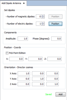
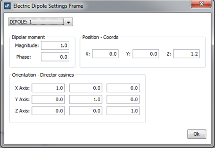
Step 4. Define an antenna over the cube clicking on Antenna → Dipole Antenna.
The position of the dipole will be (0.0, 0.0, 1.2).
Figure 5. Dipole Antenna dialog box
Figure 6. Dipole Antenna dialog box
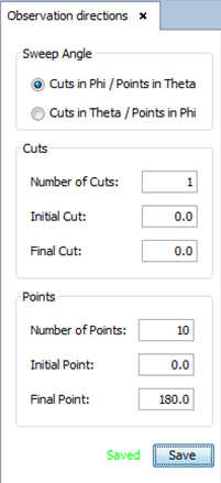
Step 5.The next step is to situate the Far Field Observation. Select
Observation directions from the Output menu. In the Angular Sweep Type dialog select
one cut in Phi = 0 degrees and 10 points in theta from 0 degrees to 360 degrees.
Select Theta as the Angular Sweeptype.
Figure 7. Far Field Observation dialog box
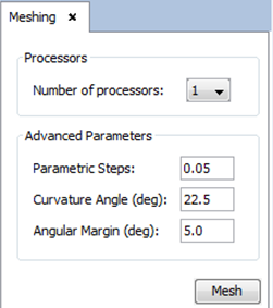
Step 6. To mesh the geometry click on Meshing → Create visibility matrix and
select the number of processors.
Figure 8. Processors option for meshing
Figure 9. Mesh
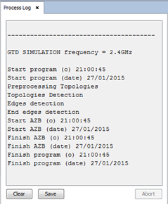
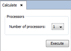
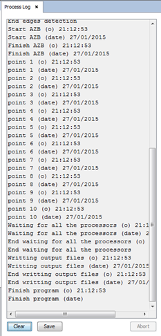
Step 7. Execute the simulation by selecting Calculate → Execute and introduce
the number of processors to be used.
Figure 10. Processors options for Execute
Figure 11. Execute
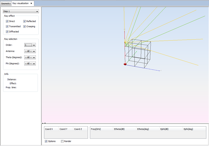
Step 8. After obtaining the results, choose view ray from show results. It is
possible to visualize order 1 rays. It is possible to represent the ray tracing
interacting with the geometry.
Figure 12. Ray Viewer dialog box
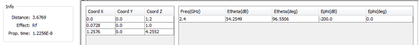
Step 9. It is possible to select a ray to show its information. Clicking in
one of the ray will fill its information in the bottom of the panel.
Figure 13. Viewing the ray information
Step 10. To visualize the charts click on Show Results → Far Field → View
Cuts, after which the following dialog will be shown: