MV-8100: Tire Modeling
In this tutorial, you will learn how to load the MBD-Vehicle Dynamics Tools preference file in MotionView, build a tire model, run the model in MotionSolve, and view the simulated results.
The purpose of this tutorial is to show the process of how to build a tire model in the MotionView interface and to interpret the results.
The tire models describe the interface between the wheel and the road. For this tire interface, the tire parameters and properties are set by a Tire Property File with the extension (.tir) while the road interface is described by a Road Property File with the extension (.rdf). One Body, one Point, and two Marker connections are needed to define the tire interface. In addition, physical properties of the tire must be specified such as: the unloaded radius, aspect ratio, width, mass, and moment of inertia's.
Load Preference File
In this step, you will launch MotionView and load the MBD-Vehicle Dynamics Tools preference file.
To build an AutoTire entity, you must first load the MBD-Vehicle Dynamics Tools preference file in MotionView. Once loaded, HyperWorks remembers and automatically loads the MBD-Vehicle Dynamics Tools preference file each time you start HyperWorks.
-
Start a new MotionView session.
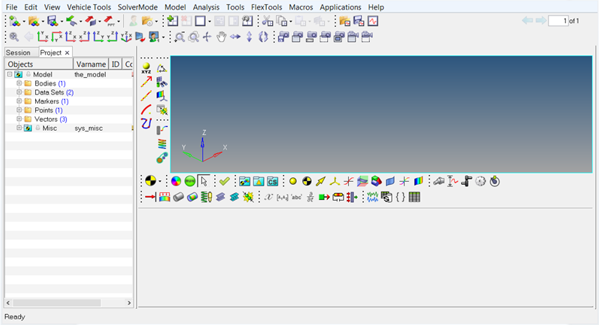 Figure 1.
 -
From the menu bar, click to open the Preferences dialog.
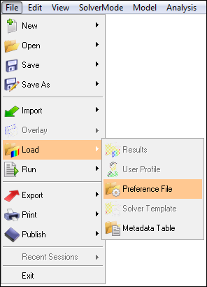 Figure 2.
 -
Select MBD-Vehicle Dynamics Tools and click
Load.
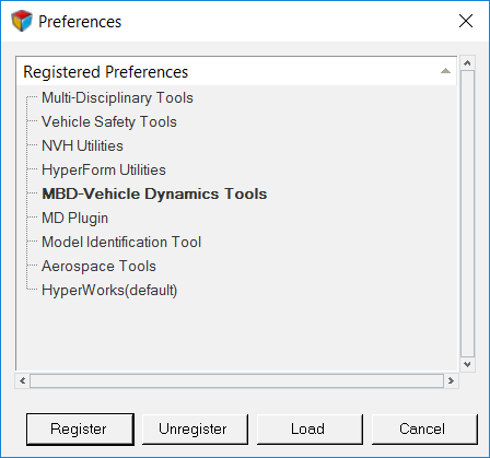 Figure 3.
Add a Point to the Model
In this step, you will add a point to the model.
-
From the Project Browser, right-click the
Points folder and select Add
Point from the context menu.
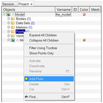
Figure 4.The Add Point or PointPair dialog opens. -
Click OK.
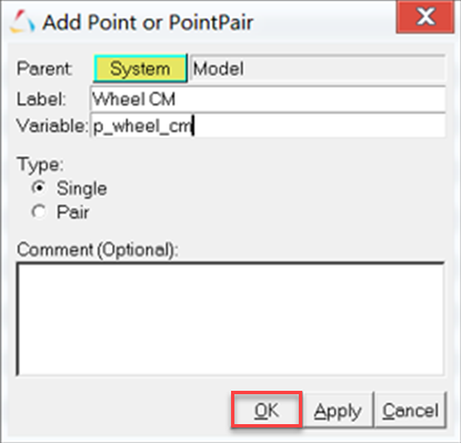
Figure 5.The Wheel CM point is added in the Project Browser.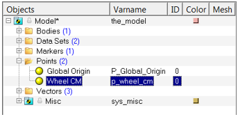
Figure 6. -
From the Points panel, enter 313 as the Z coordinate in
the Properties tab.
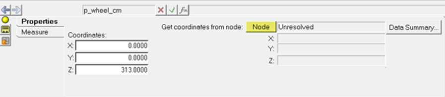
Figure 7.
Add a Hub Body to the Model
In this step, you will add a body to the model and define the center of the Hub body.
-
From the Project Browser, right-click the
Bodies folder and select Add
Body from the context menu.
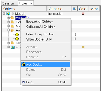
Figure 8.The Add Body or BodyPair dialog opens. -
Click OK.
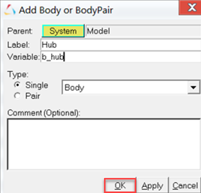
Figure 9.The Hub body is added to the Project Browser.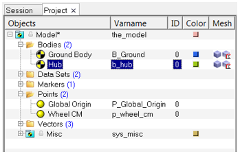
Figure 10. -
From the Body panel, click on the CM Coordinates tab and
select the Use center of mass coordinate system check
box.
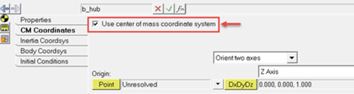
Figure 11. -
Double-click the Point collector button.
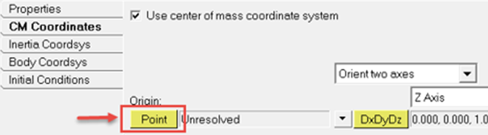
Figure 12.The Select a Point dialog opens. -
Select the Wheel CM point and click OK.
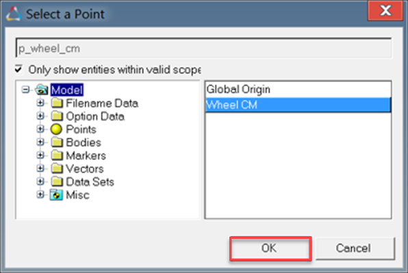
Figure 13.The center of the wheel is used as the center of the Hub body.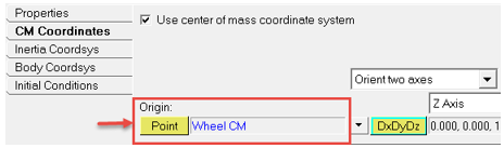
Figure 14.
Update the Mass and Inertia Properties of the Hub Body
In this step, you will update the mass and inertia properties of the Hub body.
-
For lzz, enter 1.0000e+14.
Tip: The mass and inertia properties of the Hub body should now match Figure 15.
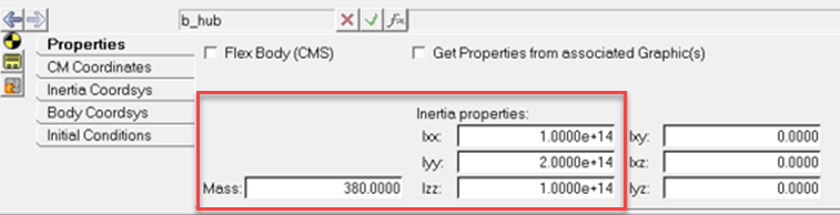
Figure 15.
Set the Initial Conditions for the Hub Body
In this step, you will set the initial conditions for the Hub body.
-
For Wz, enter 0.
Tip: The initial conditions for the Hub body should match Figure 16.
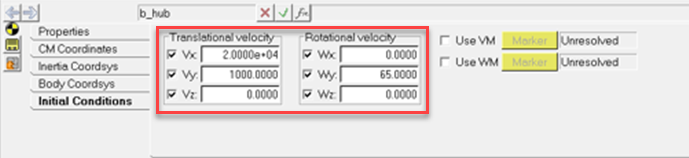
Figure 16.Note: These initial conditions applied at the Hub body represent a tire+rim with an initial forward velocity Vx of 20000mm/s and rotating at 65rad/s.
Add a Marker to the Model
In this step, you will add a marker to the model.
-
From the Project Browser, right-click the
Markers folder and select Add
Marker from the context menu.
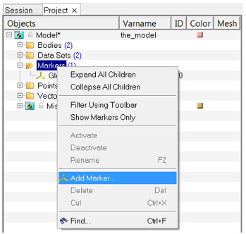
Figure 17.The Add Marker or MarkerPair dialog opens. -
Click OK.
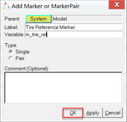
Figure 18.The Tire Reference Marker is added to the Project Browser.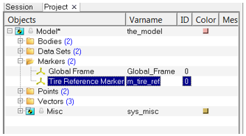
Figure 19. -
From the Markers panel, select Hub as the body and
select Wheel CM as the Origin in the Properties tab as
indicated in Figure 20.
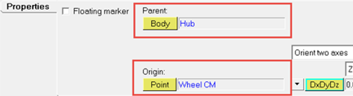
Figure 20.The attachments for the marker are defined.
Add an AutoTire Entity to the Model
In this step, you will add and autotire entity to the model.
-
From the Project Browser, right-click
Model and select Add Auto
Entity from the context menu.
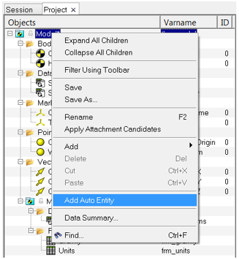
Figure 21.The Add Entity dialog opens. -
From the drop-down menu, select AutoTire and click
OK.
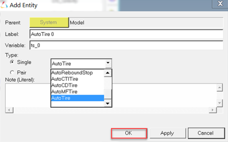
Figure 22.The AutoTire panel is displayed in the panel area and the auto entity is created in the Project Browser.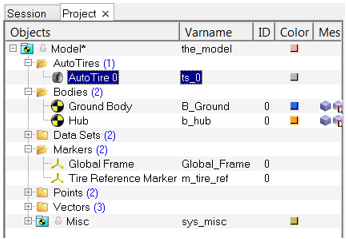
Figure 23. -
From the Connectivity tab, select Hub as Hub Body,
Wheel CM as Wheel Center, Tire Reference
Marker as Tire Marker, and Global Frame
as Road Marker as indicated in Figure 24.
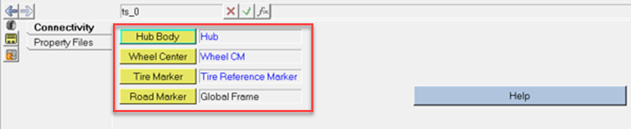
Figure 24.Note: The AutoTire is defined by a Hub Body, Wheel Center, Tire Marker, and Road Marker.- Hub Body
- The wheel body on which the tire forces act.
- Wheel Center
- Point where the tire will be attached, usually the wheel center.
- Tire Marker
- Reference marker which determines the direction in which the tire forces act.
- Road Marker
- Reference marker of the road, it is the marker with respect to which the road is positioned and oriented for the simulation.
The tire interface is defined and the tire model displays in the modeling window.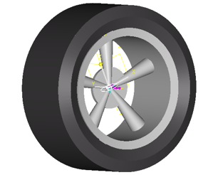
Figure 25. -
Use the Property Files tab to review the tire properties.
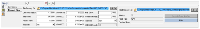
Figure 26.The AutoTire entity allows you to modify the tire properties as desired by editing the Tire Property File.
The graphic tire representation can be modifying by editing the properties field, such as Unloaded Radius, Tire Width, Aspect Ratio, and Hub Offset. Once the tire property file is loaded, some of the fields will automatically get filled.
Note: Changing the value in entry field will not change the values in tire properties file. These entry fields are meant to create the tire graphic.If you want to make changes to the file using the Edit File button, it is recommended that you save it with a different name and reload the file so that the graphic attributes are automatically filled in the graphical user interface.
Run the Model in MotionSolve
In this step, you will run the model in MotionSolve.
-
Click
 (Run Solver) and rename the
MotionSolve input to
Auto-Tire.xml.
(Run Solver) and rename the
MotionSolve input to
Auto-Tire.xml.
-
For Print interval, enter 0.001.
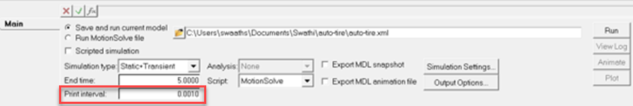
Figure 27.
View the Simulated Results
In this step, you will view the simulated results of the tire model.
-
Click the Plot button.
The plot is displayed in the right window.
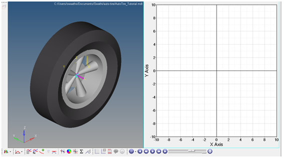
Figure 28. -
Click anywhere in the plot window and then click
 (Expand/Reduce button) from the toolbar.
The plot window expands.
(Expand/Reduce button) from the toolbar.
The plot window expands.
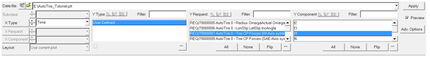
Figure 29.
- REQ/70000005 Auto Tire0 – Radius OmegaActual OmegaFree
-
- f2 - Radius – Rolling radius of the tire.
- f3 - OmegaActual – Angular velocity of the tire.
- f4 - OmegaFree – Angular velocity at which the tire will be having a zero slip ratio.
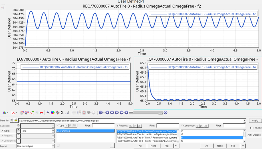
Figure 30. - REQ/70000006 Auto Tire0 – lonSlip latSlip IncAngle
- The following outputs are available in both ISO and SAE co-ordinate systems.
The one shown in plots are in ISO.
- f2 - LonSlip - Slip Ratio or Longitudinal slip in percentage. In this case the tire is rolling freely therefore the slip ratio is approximately 0.
- f3 - LatSlip - Lateral slip starts from 0.05 as lateral slip is the ratio of Vy and Vx. In our case Vy/Vx = 1000/20000 = 0.05
- f4 - IncAngle – Inclination Angle of the tire from XZ plane.
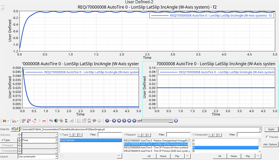
Figure 31. - REQ/70000007 Auto Tire0 – Tire CP Forces (W-Axis system)
- The Tire contact patch forces are available in both W and SAE axis system.
The one shown in plots are in W-axis System.
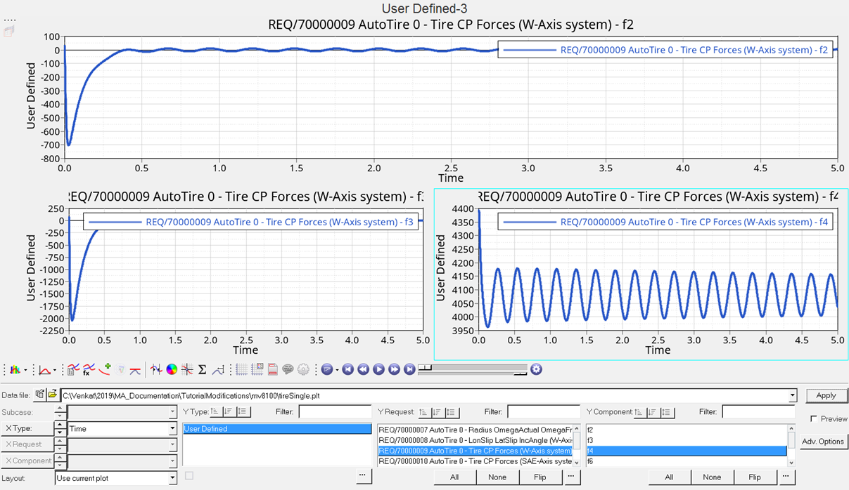
Figure 32.
Output Plot Types
In this section, you will learn about the different output plots that based on the simulation viewed in View the Simulated Results.
REQ/70000007 Auto Tire0 – Radius OmegaActual OmegaFree
- f2 - Radius – Rolling radius of the tire.
- f3 - OmegaActual – Angular velocity of the tire.
- f4 - OmegaFree – Angular velocity at which the tire will be having a zero slip ratio.
Figure 33.
REQ/70000008 Auto Tire0 – lonSlip latSlip IncAngle
The following outputs are available in both ISO and SAE co-ordinate systems. The one shown in plots are in ISO.
- f2 - LonSlip - Slip Ratio or Longitudinal slip in percentage. In this case the tire is rolling freely therefore the slip ratio is approximately 0.
- f3 - LatSlip - Lateral slip starts from 0.05 as lateral slip is the ratio of Vy and Vx. In our case Vy/Vx = 1000/20000 = 0.05
- f4 - IncAngle – Inclination Angle of the tire from XZ plane.
Figure 34.
REQ/70000009 Auto Tire0 – Tire CP Forces (W-Axis system)
The Tire contact patch forces are available in both W and SAE axis system. The one shown in plots are in W-axis System.
Figure 35.