AcuFieldView Parallel Performance Results
The degree to which certain operations in AcuFieldView Parallel will scale depends upon several factors pertaining to the dataset, and may also depend upon hardware issues as well.
| Tet Benchmark
(small) |
Tet Benchmark
(large) |
|
|---|---|---|
| File size (bytes) | 420,111,352 | 811,480,068 |
| Nodes | 2,833,166 | 5,526,084 |
| Elements | 15,540,893 | 30,374,480 |
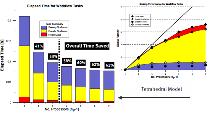
Figure 1.
Benchmark timings were obtained for the tasks of reading data, creating coordinate and iso-surfaces and sweeping these same surfaces. Overall time savings are reported as a percentage relative to the time required to complete these tasks using AcuFieldView in Client-Server mode. Using AcuFieldView Parallel with three server processes (for np values to the left of the dotted line) you should expect to see scaling improvement of 2x or better.
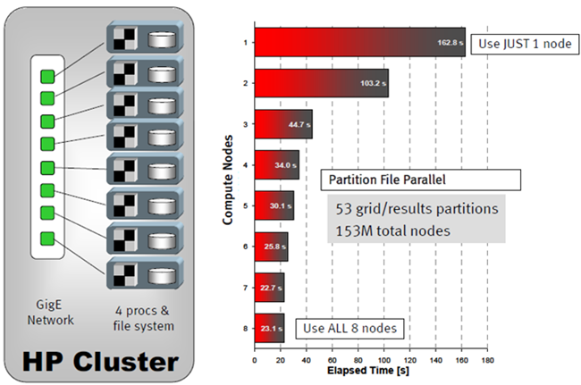
Figure 2.
Timing tests were obtained as follows. For the case of one compute node, all 53 partitions were read from the local file system on that node. For two compute nodes, the 53 partitions were spread across the file systems for two nodes, and the dataset was read again. By utilizing all eight compute nodes, a 7X reduction in the time required to read data was achieved.