NVH-1100: NVH Director Assembly
The Assembly Browser is an object oriented modeling environment where the fundamental entity is the module entity. A module is a HyperMesh entity used to represent subsystems of an assembly.
Start NVH
-
Click the Load User Profile icon,
 , on the Standard
toolbar.
, on the Standard
toolbar.
Define Assembly Hierarchy
Load an Assembly Definition XML File
-
After naming the module, you need to import an .xml file. This should be an assembly
database file that you exported from the NVH Director. Click the
 icon to navigate to a folder where the
.xml file is
located.
icon to navigate to a folder where the
.xml file is
located.
Save an Assembly Definition XML File
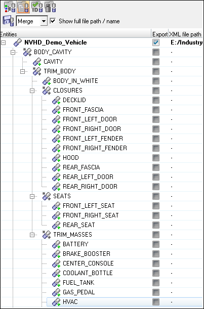
Figure 1.
Define Module Representations
-
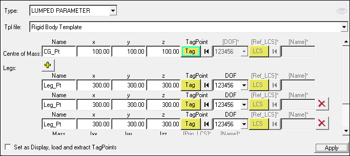
Aside from file based representations, a templated Lumped Parameter (LP)
representation can also be defined using the LP templates included in the NVH
Director, or user created templates.
-
Select one of the representations to be the active Display
 or Analysis
  representation by checking the appropriate radio
buttons.
representation by checking the appropriate radio
buttons.
Import Display Representations
-
From the Base View
 of the Assembly Browser, select the
root Module Model.
of the Assembly Browser, select the
root Module Model.
Manage TagPoints
Prepare a Module for Assembly
In the previous two steps, you have assumed that the representation file is already in an FE entity ID range that would not cause conflicts with other modules in the assembly, and all necessary tagpoints already exist in the file as 10th field comments on the respective grid cards. However, these assumptions are not met in most practical applications. Necessary preparation work needs to be done to get the module representation files to a state that is ready for assembly. This section describes how to accomplish this task.
-
Once you are finished preparing the module, you can prepare another one from
the Assembly Browser, or select to exit the Prepare Module
Mode by clicking X on the Prepare Module tab.
You will be prompted with four representation file save options with information on ID renumbering. Yes: The root representation file is to be saved, in this case, intra and inter ID conflict flag will be set to Yes. No: The root representation file is not to be saved, in this case, intra and inter ID conflict flag will be set to No. Cancel: The exit Prepare Module Mode action is aborted. No, but VALIDATE: In this case there is no change to the file and no need to save the file, but intra and inter ID conflict flag will be set to yes.
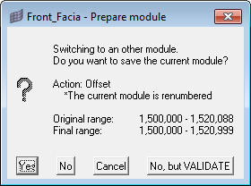
Figure 2. -
Once all of the modules have been prepared, you can review the assembly ID
ranges and conflict setting from the Id View of the Assembly Browser.
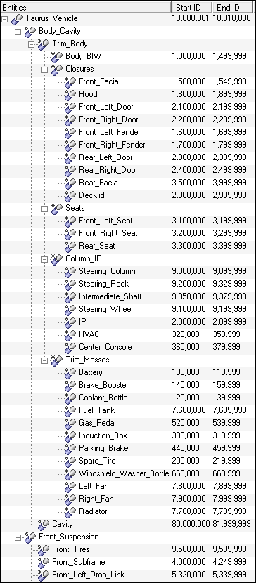
Figure 3.At the individual module level, the ID tab of the Edit Module will also be populated. It is also possible to view mass and damping information using the Property View in the Assembly Browser.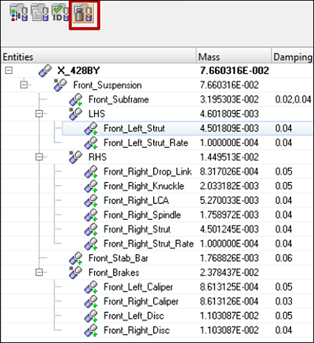
Figure 4.
Define Connections Between Modules
-
Click the
 icon to launch the connection Interactive Create
tool.
icon to launch the connection Interactive Create
tool.
-
Connections can be created between modules to be connected either by selecting
tagpoints from the list box in the dialog, or by picking tagpoints. Hint: Pick
and drag on the left hand side of the tags to ease selection off the screen
after clicking the
 icon.
You can also provide a description for the connector created, specify an owning module, a local coordinate system, connector location for the center of motion, and a collector for the connector created. Force ID's for connectors gives you an option to define the numbering pattern to a connector, so that the connection elements created by realization of those connectors fall in the defined numbering pattern. ID's are forced to connector elements and properties after realizing them.
icon.
You can also provide a description for the connector created, specify an owning module, a local coordinate system, connector location for the center of motion, and a collector for the connector created. Force ID's for connectors gives you an option to define the numbering pattern to a connector, so that the connection elements created by realization of those connectors fall in the defined numbering pattern. ID's are forced to connector elements and properties after realizing them. -
Connections can also be created using the Auto Create tool, which can be
invoked by clicking the
 icon.
Two automated creation approaches are available: auto creation by Proximity or by Tagpoint Matching.
icon.
Two automated creation approaches are available: auto creation by Proximity or by Tagpoint Matching. -
To review the connections that were created, click .
The Connector Browser is divided into two browser panes. The top pane is the Module Pane, where connected modules are listed. You can view connections attaching to modules using typical browser functions, such as Show/Hide/Isolate. The lower pane is the Connector Pane, where individual connections are listed.
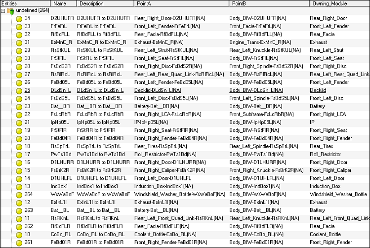
Figure 5.
Define Connection Information and Properties
-
Click Update to save the changes.
Information related to Connected Points, and distance between them, is displayed in the next section. You can modify any connecting tagpoint by clicking the
 icon next to its label, which opens the Tagpoint
Selection tool. You can then select a module first in the Module pull-down list,
select a tagpoint owned by the module, or click the icon and pick a tagpoing on the screen in the 3D
graphics window, and then click Select. The tagpoint list
can be further filtered by clicking the
icon next to its label, which opens the Tagpoint
Selection tool. You can then select a module first in the Module pull-down list,
select a tagpoint owned by the module, or click the icon and pick a tagpoing on the screen in the 3D
graphics window, and then click Select. The tagpoint list
can be further filtered by clicking the  icon and selecting one of the tagpoint types: Response,
Connection, Input, Plot, or All (default).
icon and selecting one of the tagpoint types: Response,
Connection, Input, Plot, or All (default).When checked, the Switch Nodes checkbox allows you to change the independent node from Point A to Point B, based on their dependency status, to avoid an already dependent node being specified as dependent again when the connection is realized into new rigid elements. Connection properties are defined in the States tab of the Connection Manager. The first step in defining connection properties is to select a State Set. State Set is designed to capture a unique hardware part with its own set of connection properties. For example, hydromount vs. a base rubber part. By default, a base State Set is already created and assigned to the connector. Therefore, unless there is a need for multiple sets of properties, the default base State Set selection does not need to be changed.
-
State Sets can be added by clicking the
 icon, or deleted by clicking the
  icon. You can double-click a State Set to edit its
name, and click Select to finalize the selection.
The second step in defining connection properties is to select a LCS (local coordinate system) for the properties to be defined in the next step.The following options are available in specifying coordinate systems used by any element generated during connection realization:
icon. You can double-click a State Set to edit its
name, and click Select to finalize the selection.
The second step in defining connection properties is to select a LCS (local coordinate system) for the properties to be defined in the next step.The following options are available in specifying coordinate systems used by any element generated during connection realization:- Vehicle – ‘0’ or the basic coordinate system is used.
- Owned – This option allows you to create a custom LCS by clicking Edit.
- TagPointA – Local coordinate system specified as the output Displacement Coordinate System on the grid card associated when TagPointA is used.
- TagPointB – Local coordinate system specified as the output Displacement Coordinate System on the grid card associated when TagPointB is used.
When the Owned local coordinate system is selected, a local coordinate system managed in the assembly can be created using the Define Local Coordinate System dialog. The following types of coordinate systems can be defined:- Axis-Plane – Two vectors are required to define this system. A vector can either be specified in direction cosines, or by selecting two tagpoints.
- Angle – Any combinations of angle rotations around the reference axes can be used to define this system.
- Ujoint – The Ujoint coordinate systems is defined by selecting two tagpoints on the input shaft and two tagpoints on the output shaft. A homo-kenetic coordinate system will then be created to properly describe motion transfer of Ujoints from the input to the output shafts.
The last step in defining connection properties is to define property states.The following options are available in specifying property states:- PBUSH – A CBUSH element is generated during connection realization. The PBUSH card allows you to specify K (stiffness), B (viscous damping), GE (material damping), M (mass and moment of Inertia), and RIGID (checkboxes for rigidly connected dofs.) Note: The M and RIGID fields are not supported in the Nastran profile, and are ignored.
- RIGID – A RBE2 element with dofs specified in checked boxes is generated during connection realization.
- PBUSHT – A CBUSH element is generated during connection realization. In addition to the PBUSH card that specifies the base properties, a PBUSHT card allows you to specify frequency tables for K, B, and GE.
- PBUSH-MASS – A CBUSH element with two COMN2 elements at its Point A and Point B are generated during connection realization. Note: This type is designed to be used in the Nastran profile where the M fields for PBUSH are not supported by the Nastran solver.
- PBUSH-RIGID – A CBUSH element with a parallel RBE2 element are generated during connection realization. Note: This type is designed to be used in the Nastran profile where the RIGID checkboxes for PBUSH are not supported by the Nastran solver.
-
Click Apply to save each
property state definition. Property states can also be imported using the Import
From File option by clicking the
 icon.
The Import States dialog opens.
icon.
The Import States dialog opens.
Manage Analysis
An Analysis is a collection of module, connection and loadcase selections that
completely specifies the assembly definition for a particular simulation event. The
Analysis Manager is invoked by clicking the ![]() icon.
icon.
-
To add an analysis by extracting active module and connection settings, click
the
 icon.
icon.
-
To add an analysis by copying module and connection settings from the selected
analysis, click the
 icon.
icon.
-
To add a blank analysis, click the
 icon.
The top section of the Analysis Manager is used to define analysis, which is further divided into parts. The first part is for module representation and state selection, the second is for connection state selection and the third part is for loadcase definition.
icon.
The top section of the Analysis Manager is used to define analysis, which is further divided into parts. The first part is for module representation and state selection, the second is for connection state selection and the third part is for loadcase definition. -
Highlight an existing definition or add a new one by clicking the icon.
The lower section of the Analysis Manager is used to apply the module representation and state selections to the modules in the assembly, realize connections to states defined into corresponding FE entities and render the defined loadcase into solver cards. Once an analysis has been applied, the Job options section is enabled.