Analysis of Connectivity Paths
Visualize connectivity prediction results in the 2D View and the 3D View.
Connectivity Prediction results can be visualized graphically in the 2D View and the 3D View using the Path Visualization Tool for a selected node. The path types to be shown as well as the colorization of the displayed paths can be specified on the Display tab of the Settings Dialog. Additional descriptive information for the connectivity paths of the selected node can be obtained by using the Object Information Tool.
Display of Path Types
- Path to Direct Neighbor
- Path to Gateway Node
- Optimum Path
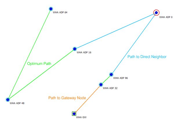
Figure 1. Example of path types.
Display of Path Loss Thresholds
User defined path loss thresholds for the path sections along the connectivity paths of a selected node can be visualized as well. The path sections are colorized according to the path loss along the path section taking into account the specified threshold values. The threshold values and the corresponding drawing color can be specified on the Display tab of the Settings dialog.
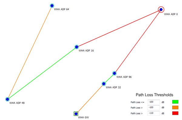
Figure 2. Example of path loss thresholds.
Display of Path Delay Thresholds
The occurring delays along the connectivity paths of a selected node can be evaluated with CoMan. The path sections are colorized according to the summed path delays along the path taking into account the specified threshold values. Starting from the selected node, the overall delay consisting of path delay and process delay of the nodes located in between is added along the path. A path section is colorized depending on the delay at the end of the section before the next node. The threshold values and the corresponding drawing color can be specified on the Display tab of the Settings dialog.
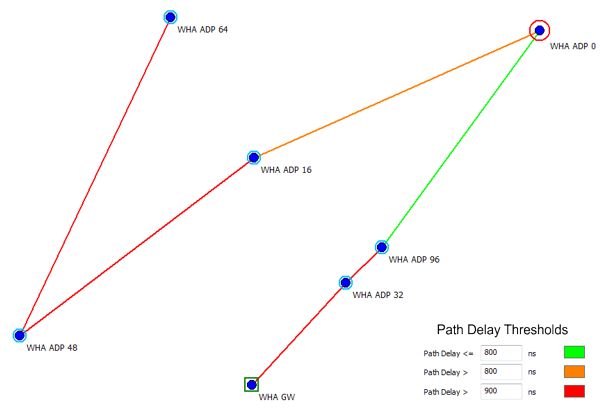
Figure 3. Example of path delay thresholds.
For example the color of the path section between node “WHA APD 16” and “WHA APD 48” is determined as follows:
Delay (at node “WHA ADP 48”) = Path delay (between nodes “WHA ADP 0” and “WHA ADP 16”)
+ Process delay (node “WHA ADP 16”)
+ Path delay (between nodes “WHA ADP 16” and “WHA ADP 48”)
As Delay (at node “WHA ADP 48”) > 900ns ==> red color