In this tutorial you will define the *STEP using the Abaqus Step Manager.
You will learn how to:
Load the Abaqus user profile
Retrieve the HyperMesh model file
Define the *STEP card and specify *STATIC as an analysis procedure
Define loads (*CLOAD) and boundary conditions (*BOUNDARY)
Define pressure loads (*DLOAD) with an element set
Define output requests
Export the database to an Abaqus input file
This exercise uses the abaqus_StepManager_tutorial.hm file, which
can be found in <hm.zip>/interfaces/abaqus/. Copy the file(s)
from this directory to your working directory.
Load the User Profile and Model
In this step you will load the Abaqus user profile and
model file.
A set of standard user profiles is included in the HyperMesh installation. User profiles change the appearance
of a panel, however they do not affect the internal behavior of each function.
Start HyperMesh Desktop.
In the User Profile dialog, set the user profile to
Abaqus, Standard
3D.
Open a model file by clicking File > Open > Model from the menu bar, or by clicking on
the Standard toolbar.
In the Open Model dialog, open the
abaqus_StepManager_tutorial.hm file.
Note: The abaqus_StepManager_tutorial.hm file contains
pre-defined model data. Use this file in the following steps to define the
history data portion of this model.
Define a *STEP Card
In this step you will create a *STEP card with the *STATIC analysis
procedure.
From the menu bar, click Tools > Loadsteps Browser.
The Step Manager opens.
Click New.
The Create New Step dialog opens.
In the Name field, type
step1.
Click Create.
A step labeled step1 opens the Load
Step dialog.
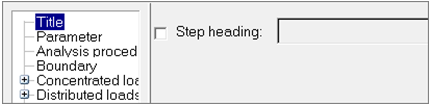
In the first pane, select Title.
The Step Heading option with a disabled field is displayed. Figure 1.
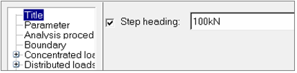
Select the Step heading checkbox and type
100kN in the text field.
Figure 2.
Click Update to store the heading information in
step1.
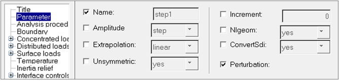
In the first pane, select Parameter.
Select the Name and Perturbation
checkboxes.
Note: Notice that Name is already set to
step1. Figure 3.
Click Update.
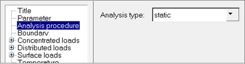
In the first pane, select Analysis procedure.
Set Analysis type to
static.
Figure 4.
Click Update.
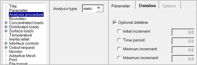
Click the Dataline tab.
Select the Optional dataline checkbox to add an
additional dataline.
Add individual data, such as Initial increment, by selecting the appropriate
checkbox and entering a value.
Note: When a checkbox is disabled, a space will be added in the ASCII file, and the Abaqus solver will use the default value. Figure 5.
Click Update.
Define Load and Boundary Conditions
In this step you will create constraints.
You will add the *CLOAD and *BOUNDARY keywords to the current load collector by
defining loads and boundary conditions.
In the first pane, select Boundary.
Click New.
The Create Load Collector dialog
opens.
In the Name field, type
loads_and_constraints.
Click Create.
Optional: In the Load collector table,
Display column, click the color icon to select a
color for the load collector.
Verify that the Status checkbox for
loads_and_constraints is selected.
Note: By selecting this checkbox, you are adding this load collector into the
loadstep.
Click the loads_and_constraints load collector.
New tabs display.
From the Define tab, verify that
Type is set to
default(disp).
Figure 6.
Click Define from 'Constraints' panel.
The Constraints panel opens, from which you will
create constraints.
Create Constraints from the Constraints Panel
In this step you will create constraints from the Constraints panel.
On the Standard Views toolbar, click (XZ Right Plane View).
In the Constraints panel, click nodes >> by
window.
With the exception of nodes at the ends of the cradle, draw a rectangle around
all of the displayed nodes.
Figure 7.
Select the exterior checkbox.
Click select entities.
HyperMesh selects all nodes outside the
window your drew. Figure 8.
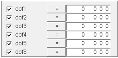
Verify that all six dof checkboxes are selected.
Figure 9.
Click create.
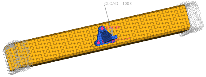
HyperMesh creates constraints at the
selected nodes. Figure 10.
Click return to go back to the Load
Step dialog.
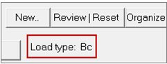
At the bottom of the Load Step dialog, look at the Load
type line.
Bc (short for BOUNDARY) appears on this line, which indicates step1 is a
load type created in the load_and_constraints load collector. The corresponding
load type in the first pane is also highlighted. Figure 11.
Create Forces
In this step you will create forces (*CLOAD).
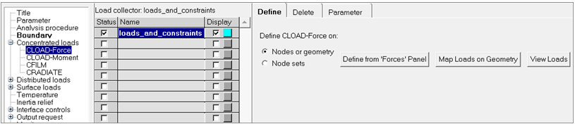
In the first pane of the Load Step dialog, expand
Concentrated loads, and select CLOAD-FORCE. New tabs
display.
Figure 12.
From the Define tab, click Define from 'Forces'
Panel.
The Forces panel opens from which you will create forces.
Create Forces from the Forces Panel
In this step you will create forces from the Forces panel.
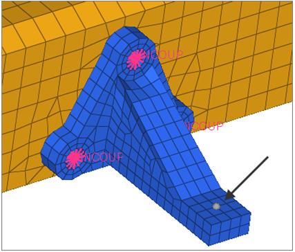
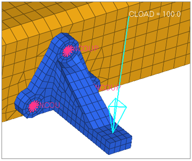
Select the central node on the top side of the bracket arm.
Figure 13.
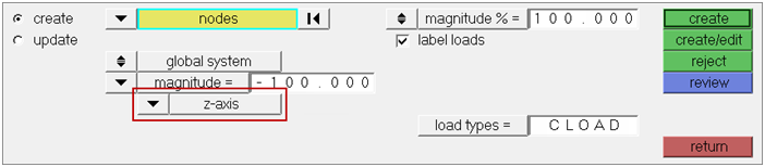
In the Forces panel, magnitude=
field, type -100.
Set the orientation selector to z-axis.
Figure 14.
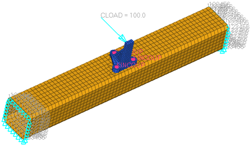
Click create.
Figure 15.
Click return to go back to the Load
Step dialog.
At the bottom of the Load Step dialog, notice the
Load type now reads Cload-f,
which indicates CLOAD-force as another load type created in the
loads_and_constraints load collector. The corresponding load type in the first
pane is highlighted.
Figure 16.
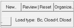
Click Review/Reset.
The constraints and forces that belong to the loads_and_constraints load
collector highlight. Figure 17.
Revert the highlighted constraints and forces to the load collector color by
right-clicking on Review.
Define Pressure Loads
In this step you will create a *DLOAD pressure load and add it to the current load
collector with an element set.
In the first pane of the Load Step dialog, expand
Distributedloads, and select DLOAD.
A new set of tabs displays.
From the Define tab, set Define DLOAD
on to Element sets.
The elements sets table displays.
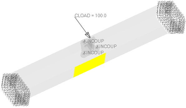
Rotate the model to the view as shown in the following image.
Figure 18.
From the Load Step dialog, set Type
to default (Pressure).
Set Element sets to
pressure_set.
Note: To view the entire list of element sets, click . Use
Fileter and Sort to narrow your search.
Click the right arrow to add the selected set to the element sets table.
Figure 19.
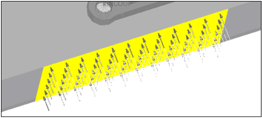
Under Element sets, click Review | Reset
Set. The element set highlights.
Figure 20.
Revert the load collector back to its original color by right-clicking on
Review | Reset Set.
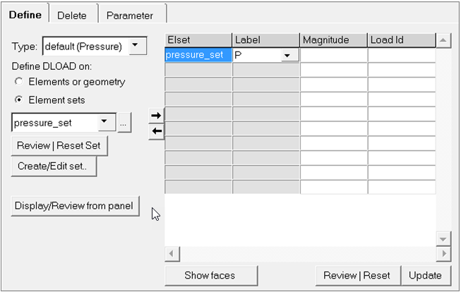
In the element sets table, Label column, select
P for the newly added
pressure_set.
Figure 21.
Because the pressure_set contains shell elements, the
direction of normal to the elements must be known to determine the sign of the
magnitude. Find the direction of the normal by selecting the
pressure_set element from the table and clicking
Show faces.
Figure 22.
Clear the display by right-clicking on Show faces.
In the element sets table, Magnitude column, type
-10 for pressure_set.
Note: The negative magnitude means pressure load in the opposite direction of
the underlying shell element normals.
Click Update.
The HyperMesh database updates. The
Load type line, at the bottom of the dialog, now
displays Dload, which indicates DLOAD as another load type created in the
loads_and_constraints load collector. The corresponding load type is the first
pane is also highlighted. Figure 23.
In the element sets table, Elset column, click
pressure_set.
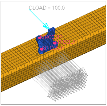
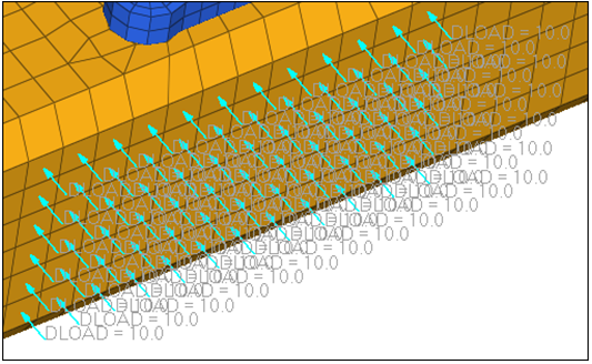
Click Review | Reset Set to review the loads.
Figure 24.
Revert back to the standard view by right-clicking on Review | Reset
Set.
Figure 25.
In this exercise, you constrained and applied distributed loads on the model
using HyperMesh panels. The loads (*DLOAD)
information is automatically stored in step1. Next,
you will specify the output requests for this step.
Request ODB File Outputs
In this step you will specify several output requests for
step1.
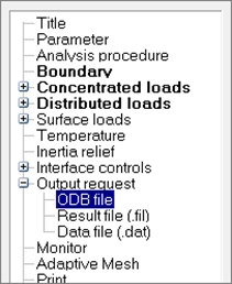
In the first pane of the Load Step dialog, expand
Output request and click ODB
file.
Figure 26.
Click New.
In the Create Output block dialog,
Name field, type step1.
Click Create.
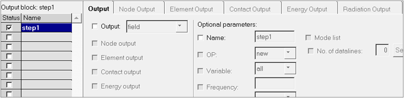
In the Output block table, click
step1.
New tabs appear. Figure 27.
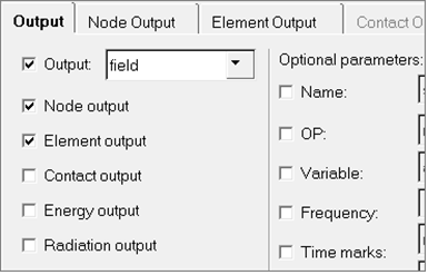
In the Output tab, select the
Output checkbox. Leave Output
set to field.
Select the Node output and Element
output checkboxes.
the Node Output and Element
Output tabs become active. Figure 28.
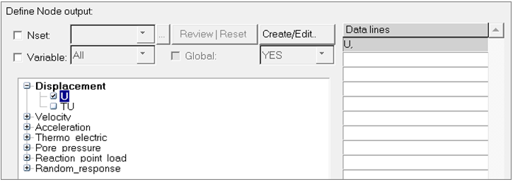
Click the Node Output tab.
Expand Displacement and select U.
The Data lines table now displays "U", which
allows you to request displacement results obd in the
file.
Note: You can manually type output request into the Data
lines table, including unsupported requests. They will be
written just as they are entered in the table. Figure 29.
Click Update.
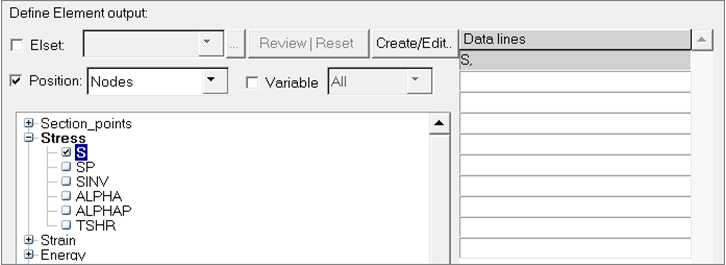
Click the Element Output tab.
Select the Position checkbox and set it to
Nodes.
Expand Stress and select S.
The Data lines table now displays "S" which
allows you to request stress results in the .obd file. Figure 30.
Click Update.
Request Result File Outputs
In this step you will request results file (.fil)
outputs.
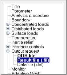
In the first pane of the Load Step dialog, expand
Output request and click Result file
(.fil).
Figure 31.
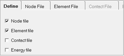
In the Define tab, select the Node file and
Element file checkboxes.
The Node File and Element File tabs become active.Figure 32.
Click the Node File tab.
Expand Displacement and select
"U."
The Data lines table displays "U," which allows you to request
displacement result in the .fil file.
Click Update.
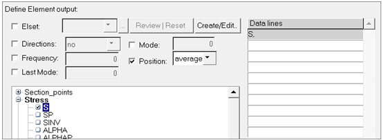
Click the Element File tab.
Select the Position checkbox and set it to
averaged at nodes.
Expand Stress and select S.
The Data Line table displays "S," which allows you to request str4ess
results in the .fil file. Figure 33.
Click Update.
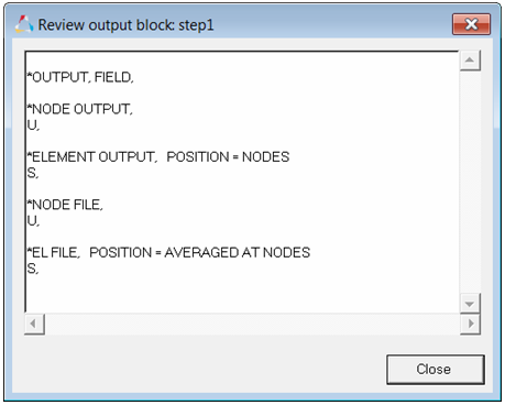
Under the Output block table, click Review | Reset.
The Review output block dialog opens and displays
the output requests you made.
Note: This is the format used in the Abaqus input file (.inp). Figure 34.
Click Close to exit the Review output
block dialog.
In the first pane of the Load Step dialog, click
Unsupported cards.
Optional: Select the Unsupported cards checkbox to add any
unsupported card.
Click Close to exit the Load Step
dialog and return to the Step Manager.
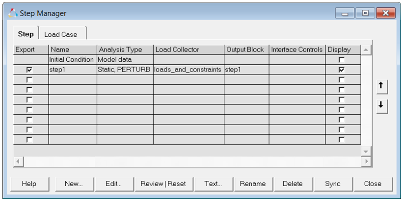
The Step Manager dialog displays all information
you defined for step1. Figure 35.
Click Close to exit the Step
Manager dialog.
Export the .inp File
In this step you will export the .inp file.
The data currently stored in the database must be output to an Abaqus.inp file for use with the Abaqus
solver. The .inp file can then be used to perform the analysis
using Abaqus outside of HyperMesh.
From the menu bar, click File > Export > Solver Deck.
In the File: field, type job1.inp.
To the left of Export Options, click .
Set Export to all.
Click Export.
Save the .hm File
In this step you will save the .hm
file.
From the menu bar, click File > Save as > Model.
In the Save Model As dialog, type
job1.hm as the file name.
Click Save.
Notes:
After you quit HyperMesh, you can run the
Abaqus solver using the
job1.inp file that was written from HyperMesh.
At your site, you can use the Abaqus license
to run this model.
If the batch mode option is being used, then enter the name of the
.inp file
exported in the previous step as the input file.
After you have successfully completed the analysis, the result file will
be available in your working directory with the name
<jobname.odb>.
Use HvTrans to translate the Abaqus solver
result file to an H3D file.
Open HyperView from the Application Menu
In this step you will open HyperView from the application
menu.
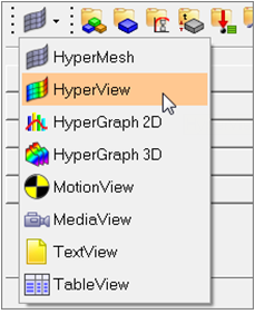
On the Client Selector toolbar, select HyperView.
HyperView opens.
Figure 36.
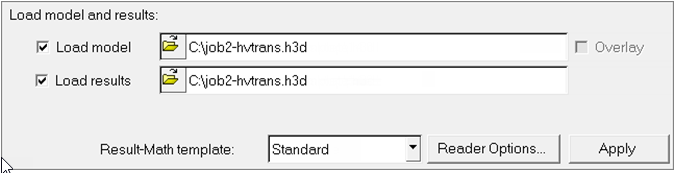
In the panel area, load the model and results
files.
Note: Load *.h3d files for both the model and result
files. Figure 37.
Click Apply.
On the Results toolbar, click
to open the Contour panel.
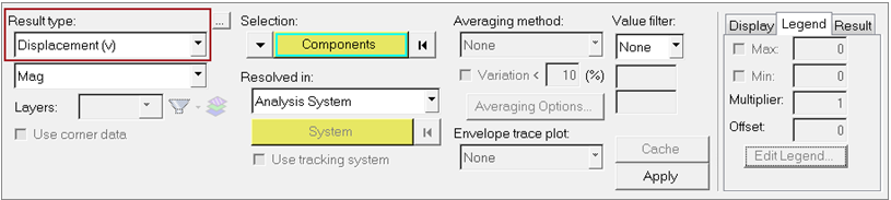
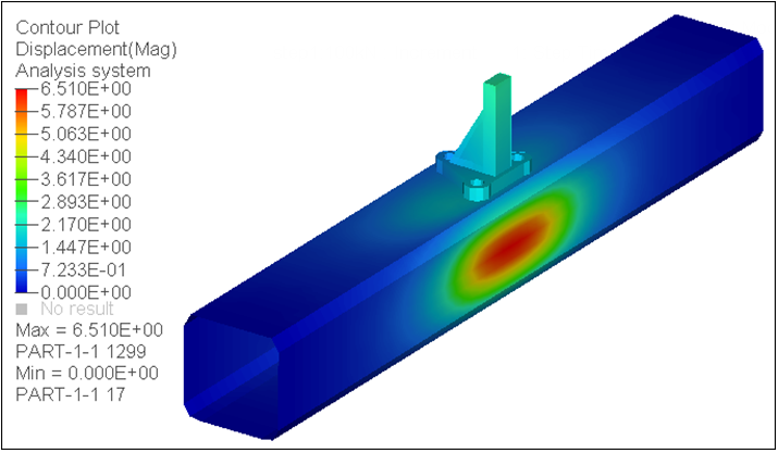
Review displacement (v) results by setting the Result
type to Displacement (v).
Figure 38.
Click Apply.
Figure 39.
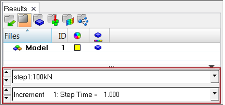
In the Results Browser, review steps and increments.
Figure 40.
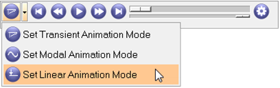
On the Animation toolbar, set the animation mode to
linear.
Figure 41.
Review the animation by clicking .
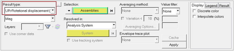
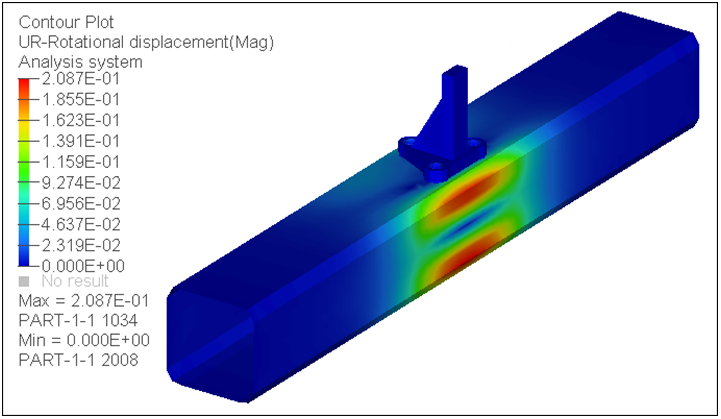
Review UR-Rotational displacement (v) results by setting the Result type to
UR-Rotational displacement (v) in the Contour panel.
 on
the Standard toolbar.
on
the Standard toolbar.

 (XZ Right Plane View).



 . Use
Fileter and Sort to narrow your search.
. Use
Fileter and Sort to narrow your search.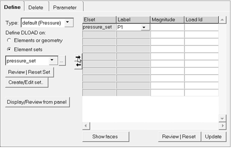
 .
.
 to open the Contour panel.
 .
.