ACU-T: 5100 Modeling of a Fan Component: Axial Fan
Prerequisites
This simulation provides instructions for running a steady state simulation of flow inside a pipe with an interior fan placed at the middle of the pipe. Prior to starting this tutorial, you should have already run through the introductory tutorial, ACU-T: 1000 HyperWorks UI Introduction, and have a basic understanding of AcuSolve and HyperMesh. To run this simulation, you will need access to a licensed version of HyperMesh and AcuSolve.
Prior to running through this tutorial, copy HyperMesh_tutorial_inputs.zip from <Altair_installation_directory>\hwcfdsolvers\acusolve\win64\model_files\tutorials\AcuSolve to a local directory. Extract ACU-T5100_AxialFanComponent.hm and AxialCoefficient.txt from HyperMesh_tutorial_inputs.zip.
Since the HyperMesh database (.hm file) contains meshed geometry, this tutorial does not include steps related to geometry import and mesh generation.
Problem Description
The problem to be solved in this tutorial is shown schematically in the figure below. It consists of an interior fan which rotates at a speed of 377 rad/sec (~3600 RPM) and has a thickness of 0.06 m and a tip radius of 0.11 m. The volumetric flow rate at the inlet is 0.146 m3/sec (~525.35 m3/hr). The problem is simulated as a steady state run and the pressure rise across the fan region is computed.

Figure 1.
Open the HyperMesh Model Database
-
Click the Open Model icon
 located on the standard toolbar.
The Open Model dialog opens.
located on the standard toolbar.
The Open Model dialog opens.
Set the General Simulation Parameters
-
Ensure that the Analysis type is Steady State.
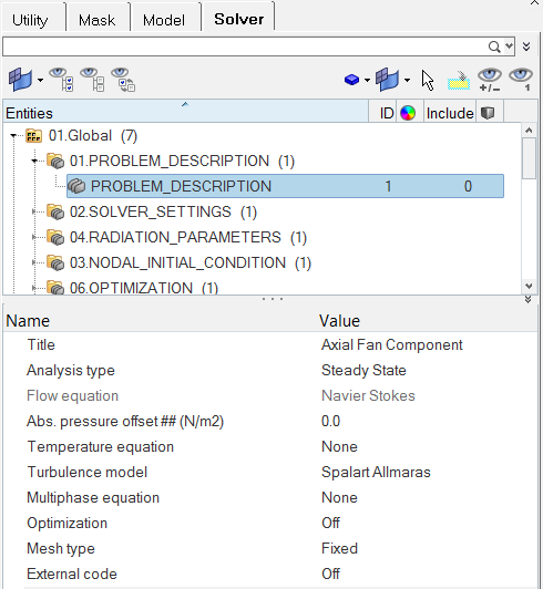
Figure 2.
Set the Boundary Conditions
-
Click Inlet. In the Entity Editor,
- Change the Type to INFLOW.
- Set the Inflow type to Flow rate.
- Set the Flow rate 0.146 m3/sec.
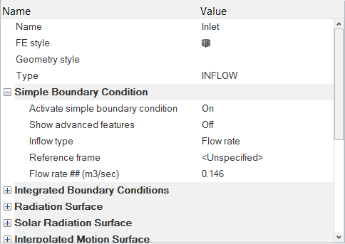
Figure 3. -
Click Fan_Inlet. In the Entity Editor,
- Change the Type to FAN_COMPONENT.
- Set the Rotational speed to 377 rad/sec.
- Set the Tip radius to 0.11 m.
- Set the Fan thickness to 0.06 m.
- Change the Axial coefficient type to Piecewise Bilinear.
- For the Axial coefficient curvefit file, click the open file icon and browse to the location where you saved AxialCoefficient.txt and select it. Click Open.
- Verify that the Radial coefficient and Tangential coefficient are set to 0.
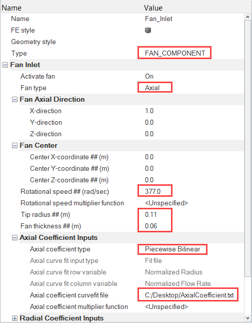
Figure 4. -
Click Outlet. In the Entity Editor, change the Type to OUTFLOW.
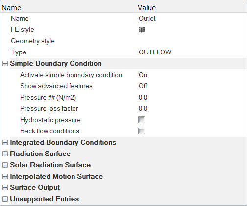
Figure 5. -
Click Walls. In the Entity Editor, verify that the Type is set to WALL.
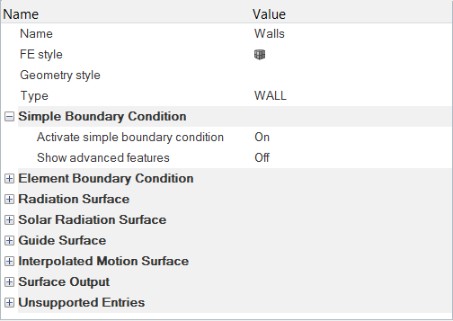
Figure 6.When component type is assigned as Wall, all the elements in the surface set are automatically re-grouped into surface sets based on the parent volume they belong to and also if they are internal or external. Auto_Wall is an advanced feature in AcuSolve which takes care of this process internally, without you having to do it manually and hence reducing the number of steps in the workflow.
-
Click Downstream_Duct. In the Entity Editor,
- Change the Type to FLUID.
- Select Air_HM as the Material.
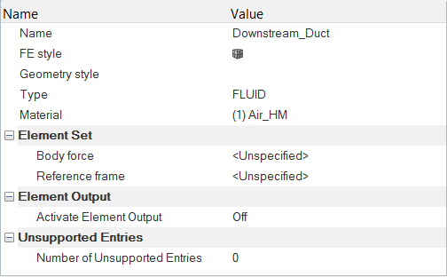
Figure 7.
Compute the Solution
In this step, you will launch AcuSolve directly from HyperMesh and compute the solution.
Run AcuSolve
-
Click
 on the ACU toolbar.
The Solver job Launcher dialog opens.
on the ACU toolbar.
The Solver job Launcher dialog opens. -
Leave the remaining options as
default and click Launch to start the solution
process.
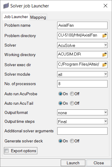
Figure 8.
Post-Process with AcuProbe
As the solution progresses, the AcuProbe window is launched automatically. AcuProbe can be used to monitor various variables over solution time.
-
Right-click on Final and select Plot
All.
Note: You might need to click
 on the toolbar in order to
properly display the plot.
on the toolbar in order to
properly display the plot.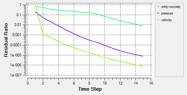
Figure 9. -
Click the User Function icon
 from the toolbar.
-
In the Function field of the User Function dialog, type
Fan_In = then paste the name you just copied.
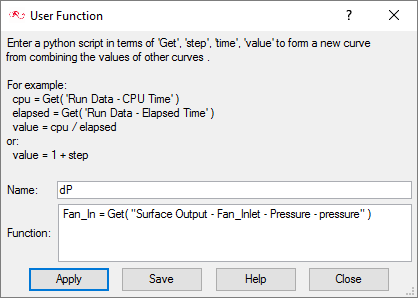
Figure 10. -
Paste the name in the Function field after Fan_Out =.
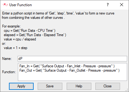
Figure 11. -
On a new line, type value = Fan_Out - Fan_In.
Note: The word “value” is case sensitive and should always be in lower case. If you use a capital letter, an error window appears.
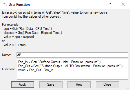
Figure 12. -
In the Data Tree, expand User
function then right-click on dP and
select Plot.
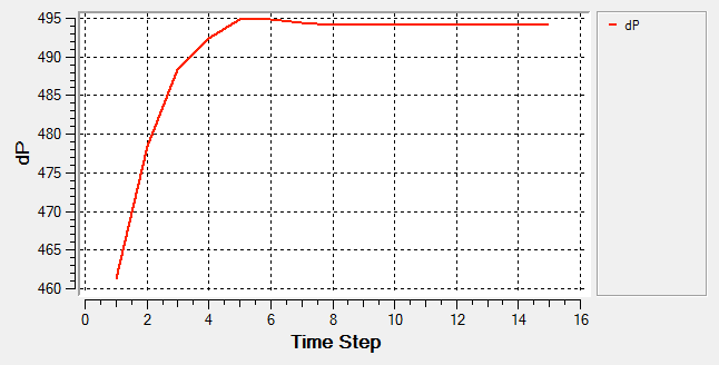
Figure 13.You can zoom into the plot by clicking
 then selecting an area at the end of the curve. As shown in the figure
below, for the given flow rate of 525.35 m3/hr (0.146
m3/sec), the pressure rise is 494.182 Pa.
then selecting an area at the end of the curve. As shown in the figure
below, for the given flow rate of 525.35 m3/hr (0.146
m3/sec), the pressure rise is 494.182 Pa.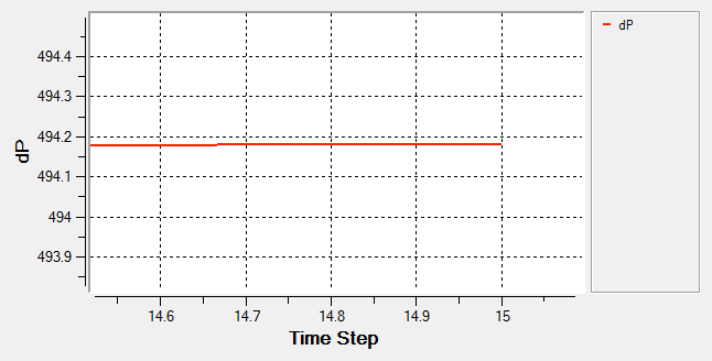
Figure 14.
Summary
In this tutorial you successfully learned how to set up and solve a simulation involving a fan component. You imported the meshed geometry and then assigned the material properties and boundary conditions to all the regions. Once the solution was computed, you defined a user function to create a plot of the pressure rise across the fan component volume.