ACU-T: 5001 Blower - Transient (Sliding Mesh)
Prerequisites
This tutorial provides the instructions for setting up, solving, and viewing results for a transient simulation of a centrifugal air blower utilizing the sliding mesh approach. In order to run this tutorial, you should have already run through ACU-T: 5000 Centrifugal Air Blower with Moving Reference Frame (Steady) and kept the solution in your working directory. It is assumed that you have some familiarity with HyperMesh, HyperMesh, and HyperView.
Prior to running through this tutorial, copy HyperMesh_tutorial_inputs.zip from <Altair_installation_directory>\hwcfdsolvers\acusolve\win64\model_files\tutorials\AcuSolve to a local directory. Extract ACU-T5001_BlowerTransient.hm from HyperMesh_tutorial_inputs.zip.
Since the HyperMesh database (.hm file) contains meshed geometry, this tutorial does not include steps related to geometry import and mesh generation.
Problem Description

Figure 1.
Open the HyperMesh Model Database
-
Click the Open Model icon
 located on the standard toolbar.
The Open Model dialog opens.
located on the standard toolbar.
The Open Model dialog opens.
Run the Steady State Simulation
-
Click
 on the ACU toolbar.
The Solver job Launcher dialog opens.
on the ACU toolbar.
The Solver job Launcher dialog opens.
Set the Transient Simulation Parameters
Set the General Simulation Parameters
-
Set the Mesh type to Fully Specified.
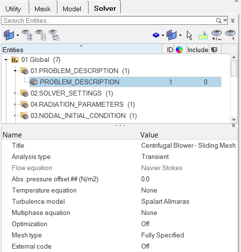
Figure 2.
Specify the Solver Settings
-
Change the Relaxation factor to 0.
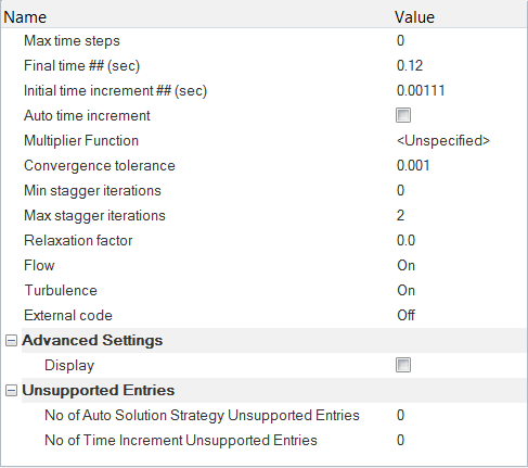
Figure 3.
Set the Nodal Output Frequency
-
Turn On the Output initial condition field.
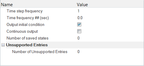
Figure 4.
Define Mesh Motion and Set Up Boundary Conditions
Create Mesh Motion
-
Set the Angular velocity - Z to -157.08 rad/sec.
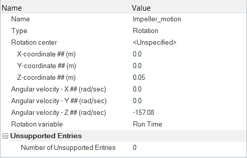
Figure 5.
Modify the Boundary Conditions
-
Click Fluid_Impeller. In the Entity Editor,
- Set the Reference frame to Unspecified.
- Set the Mesh motion to Impeller_Motion.
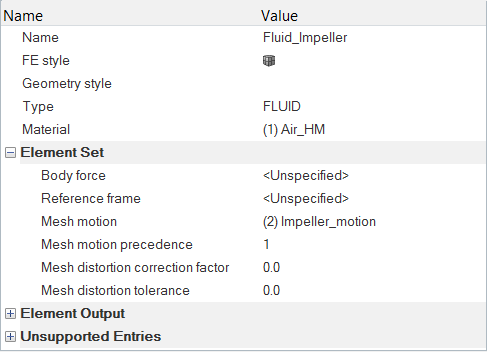
Figure 6.
Specify the Nodal Initial Conditions
-
In the Entity Editor, under the Pressure tab,
- Set the Type to Nodal Values.
- Change Select nodes by to NIC file.
- Click the open file icon in the NIC file field and browse to the HYPERMESH.DIR folder located in your working directory. Select the file Blower_Transient.pres.nic.
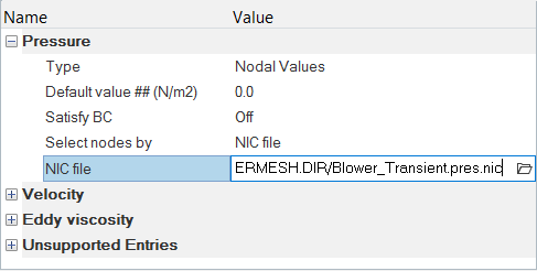
Figure 7.
Compute the Solution
-
Click on the ACU toolbar.
The Solver job Launcher dialog opens.
-
Leave the remaining options as
default and click Launch to start the solution
process.
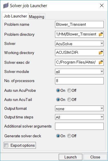
Figure 8.Once the solution is launched, the AcuSolve Control tab opens. Also, the AcuTail and AcuProbe windows are launched automatically in which the solution progress can be monitored.
Post-Process the Results with HyperView
Open HyperView and Load the Model and Results
-
In the Load model and results panel, click
 next
to Load model.
next
to Load model.
Create a Pressure Animation
-
Click
 on the Results toolbar to open the Contour panel.
-
In the panel area, under the Display tab, turn off
the Discrete color option.
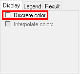
Figure 9. -
Click the Legend tab then click Edit
Legend. In the dialog, change the Type to Dynamic
scale and the Numeric format to Fixed
then click OK.
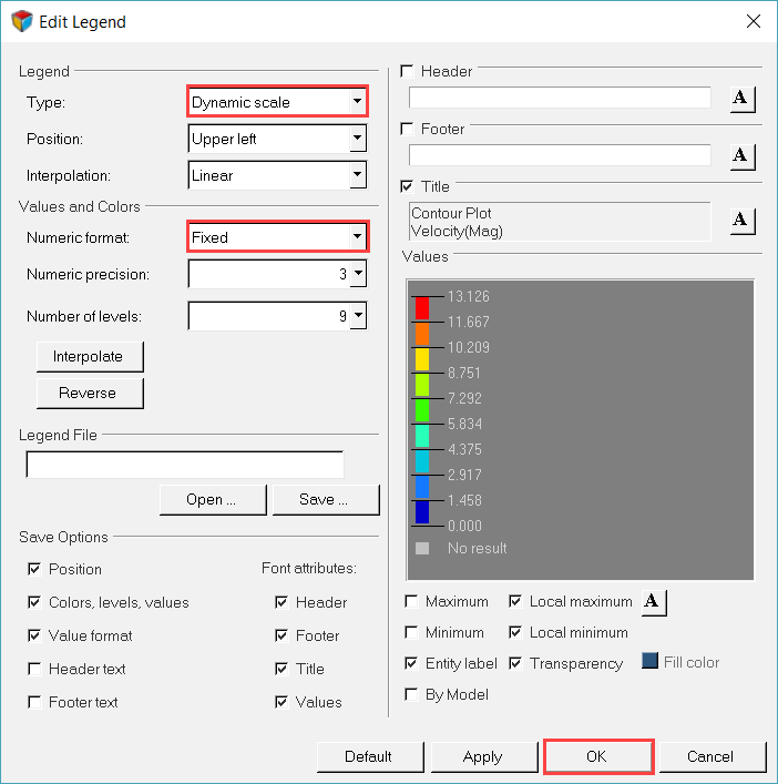
Figure 10.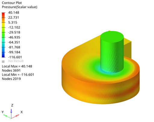
Figure 11. -
Click
 on the Display toolbar to open the Section Cut
panel.
on the Display toolbar to open the Section Cut
panel.
-
Click Girdline.... In the dialog, turn off the
Show Grid Line option then click
OK.
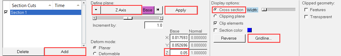
Figure 12. -
Orient the display to the xy-plane by clicking
 on the Standard Views toolbar.
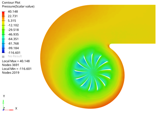
Figure 13. -
From the Animation toolbar, click the Animation controls
icon.

Figure 14. -
Click on the Start/Pause Animation icon to play the
velocity magnitude animation.

Figure 15.
Create Streamlines
-
Click on the Display toolbar to open the Section Cut
panel.
-
In the Results Browser, expand the list of
Components and turn off all components except the
Inlet, Outlet, AUTO
Fluid_Main wall and AUTO Fluid_Impeller
wall.
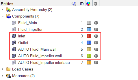
Figure 16. -
Change the element display mode to Transparent Elements and Feature
Lines.
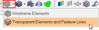
Figure 17. -
Click Apply to plot the velocity magnitude.
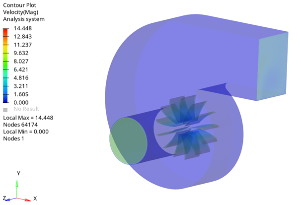
Figure 18. -
Click
 on the Results toolbar to open the Streamlines
panel.
on the Results toolbar to open the Streamlines
panel.
-
Toggle on the Draw as tube checkbox then click
Create Streamlines to generate the streamlines.
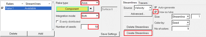
Figure 19.This will generate streamlines originating from the Inlet surface with seeds that are distributed over the surface area of the fan blades and end at the outlet.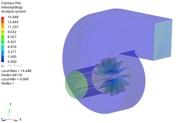
Figure 20. -
Leave the other default values unchanged then click
Create to generate the tracers.
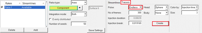
Figure 21.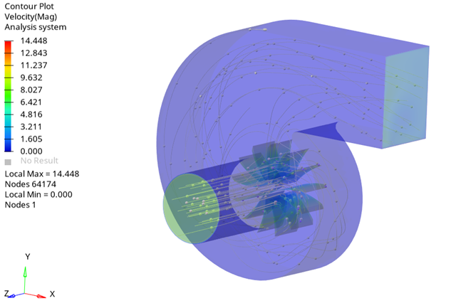
Figure 22.
Summary
In this tutorial, you successfully learned how to set up and solve a transient simulation of a centrifugal air blower using the sliding mesh approach. You started by importing the meshed geometry and then ran the steady state simulation. Then, you used the steady state result as the starting point for the transient simulation using the AcuProj tool to specify the nodal initial conditions and then solved the transient simulation using the sliding mesh approach instead of the moving reference frame approach. Once the transient solution was computed, you launched HyperView and created an animation of pressure contours and streamlines.