Set Up an AcuSolve Input Deck
The following section describes the set up of an AcuSolve input deck within Engineering Solutions.
Import an Existing AcuSolve Model
Figure 1.
Load the CFD User Profile and Open the Solver Browser
-
Click the
 icon on the
Standard toolbar.
icon on the
Standard toolbar.
- Select in the User Profiles dialog.
- Click .
Create CFD Components
-
Using the Organize panel, you can move elements to the appropriate
components.
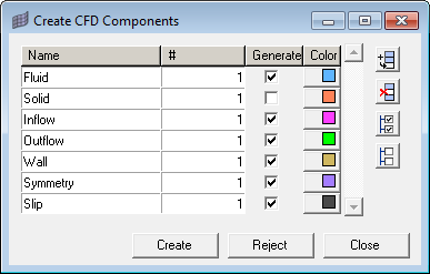
Figure 2.
Set Up the Model in the Solver Browser
The Solver Browser can be used to set up a case to run CFD analysis using AcuSolve.
It is useful for setting up problems with simple boundary conditions. For more complex problems, export the model and set it up in AcuConsole.
| Global | This folder is used to define problems and set solver parameters for that problem. It contains the following sub folders: Nodal Initial Condition, Problem Description, Radiation Parameters and Solver Settings. The Problem Description folder contains utilities to set up the analysis type and solver models. Use the Solver Settings folder to define parameters related to selected analysis types and solver models. Initial condition can be defined in the Nodal Initial Condition folder. The radiation parameters for the model can be defined in the Radiation Parameters folder. |
| Output | Define the frequency of different outputs: Derived Quantity Output, Nodal Output and Restart Output. |
| Volumes | Components with Fluid and Solid card images are grouped in this folder. |
| Surfaces | Components with Inflow, Outflow, Wall, Slip, Symmetry and Far Field card images are grouped in this folder. |
| Components With No Card Image | Components with no card image will not be exported with the solver deck. By default, all of the components will not have a card image. You have to choose the appropriate card image for the component and the component will be moved to the Surfaces or Volumes folder accordingly. |
| Nodal Boundary Condition | Define boundary conditions on nodes apart from surface boundary conditions. |
| Materials | Define/edit the material model for CFD analysis. |
| Body Force | Define gravity and heat source for volume components. |
| Periodic Boundary Condition | Define periodic or axisymmetric boundaries along with the transformation definition. |
| Reference Frame | Define reference frames. |
| Mesh Motion | Define mesh motion. |
| Emissivity Model | Define emissivity model for radiation. |
| Multiplier Function | Define multiplier functions to ramp up supported parameters. |
| Parameter | Parameters can be utilized to run solver parameter based
studies. For example, if you want to run a series of simulations with inlet velocity values of 0.5 m/s, 0.75 m/s, 1 m/s respectively, you can define a parameter on inlet velocity with the desired values. Using the HyperStudy Job Launcher DOE studies can be performed. |
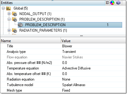
Figure 3.
Define Component Type/Properties
-
Click the component and edit it in the Entity Editor.
The elements are grouped into components of a specific type. By default, all components will have None card image and will appear in the Components With No Card Image folder. You have to choose the appropriate card image for the component and the component will be moved to the Surface or Volume folder accordingly. There are eight types of components: FLUID, SOLID, INFLOW, OUTFLOW, WALL, SLIP, SYMMETRY and Far Field. Each component in the model needs to be assigned to one of those types. For INFLOW, OUTFLOW, WALL and SYMMETRY there are four categories: Simple Boundary Condition, Radiation Surface, Interface Surface and Surface Output. Each category can be turned on or off.
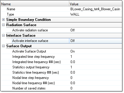
Figure 4.
Define Nodal Boundary Condition
This folder can be used to define boundary conditions on nodes apart from simple boundary conditions.
-
Right-click Nodal_Boundary_Condition and select
Create.
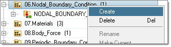
Figure 5.
Create Material Model
The Materials entity is used to define/edit the material model for CFD analysis.
- Aluminum
- Air
- Water
-
Right-click Materials and select or Material(Solid).
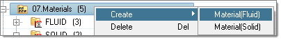
Figure 6.
Create Body Force
This folder can be used to define gravity and heat source for volume components.
-
Right-click Body_Force and select Create.
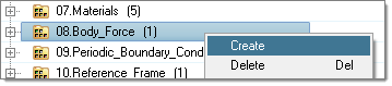
Figure 7.
Create Periodic Boundary Condition
This folder can be used to define periodic boundary condition.
-
Right-click Periodic_Boundary_Condition and select
Create.
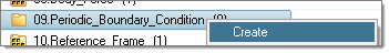
Figure 8.
Create Reference Frame
This folder can be used to define reference frames.
-
Right-click Reference_Frame and select Create.
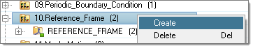
Figure 9.
Create Mesh Motion
This folder can be used to define mesh motion.
-
Right-click Mesh_Motion and select Create.
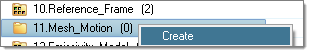
Figure 10.
Create Emissivity Model
This folder can be used to define emissivity model for radiation.
-
Right-click Emissivity_Model and select Create.
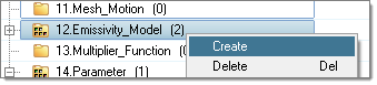
Figure 11. -
Assign emissivity to the model.
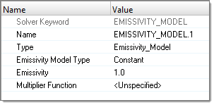
Figure 12.
Create Multiplier Function
-
Right-click Multiplier_Function and select Create.
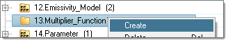
Figure 13. -
Define the Multiplier Function Type as Constant, Piecewise Linear, Cubic Spline
or Piecewise Log Linear.
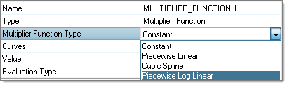
Figure 14. -
If you select Piecewise Linear, Cubic Spline or Piecewise Log Linear,
right-click on to create a new plot for the curve definition.
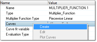
Figure 15. -
Right-click on .
The Curve editor opens.
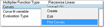
Figure 16. -
Edit the plot values, click Update to visualize the plot
and then close the Curve Editor.
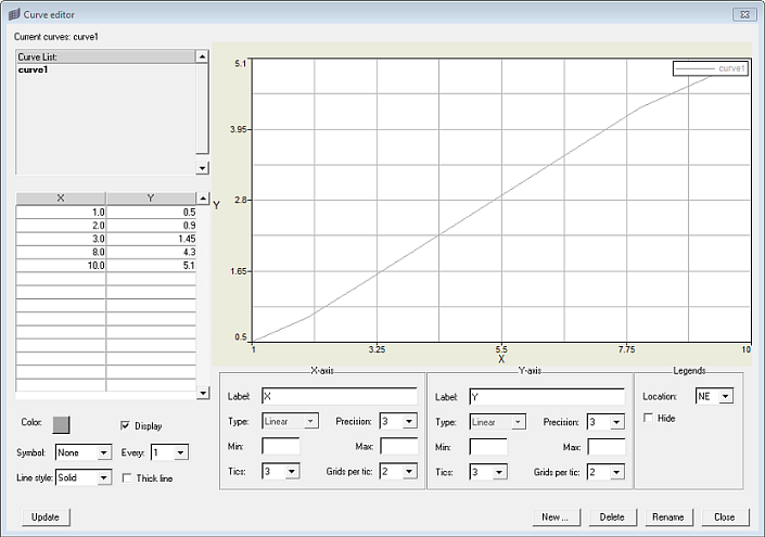
Figure 17. -
Assign the multiplier function to one of the supported fields: reference frame,
mesh motion, emissivity model or material properties (viscosity and
conductivity).
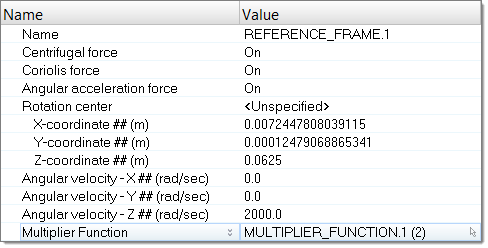
Figure 18.
Create Parameter
This folder can be used to define parameters for Solver parameter based studies.
-
Right-click Parameter and select Create.
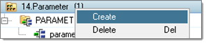
Figure 19. -
Define the Parameter mode and the Parameter type. Two parameter modes are
available: Discrete and Continuous. Discrete refers to the input values list.
You have to first define how many counts you want to define, and then click on
the table to define the values.
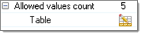
Figure 20.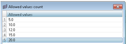
Figure 21.Continuous refers to incremental values defined by Lower bound, Upper bound and No of levels.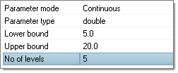
Figure 22. -
Assign the defined parameter to the solver variable input by right clicking .
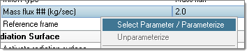
Figure 23.Note: If the solver variable accepts double values only parameters with double type will be filtered out for selection.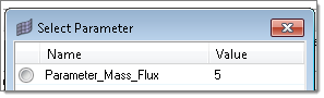
Figure 24.
Launch the Solver Run
-
Invoke the Solver job Launcher by clicking the
 icon in the CFD
toolbar. In the dialog, define the Problem name and specify the Problem
directory, which contains the solver input file.
icon in the CFD
toolbar. In the dialog, define the Problem name and specify the Problem
directory, which contains the solver input file.
-
Clicking Launch starts the Solver run.
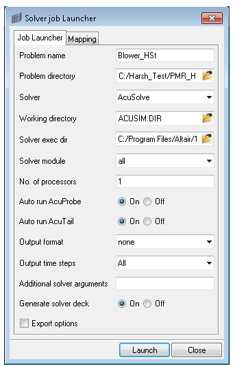
Figure 25.By default Auto run AcuProbe and Auto run AcuTail are activated, which will invoke AcuTail to monitor the .log file and AcuProbe to monitor the residuals of the current run. Both utilities access the .log file of a solver run.
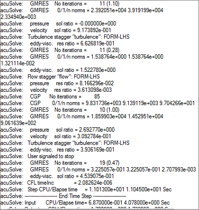
Figure 26.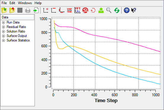
Figure 27.