Deviation Metrics Calculations
The Sprague-Geers method is a robust way to gauge the similarity between two sets of curves.
A value close to 1.0 indicates a very close similarity between the curves and 0.0 indicates much dissimilarity between them. The measure takes into consideration all available data points and therefore represents the behavior of the entire set of data. The measure however is abstract, and visualizing the Sprague-Geers metric is difficult. For instance, what does a metric of 0.75 mean? You can only gauge this by plotting the curves.
Deviation Metric
In order to address the challenges of the Sprague-Geers method, you have to understand the deviation metric. This metric is very simple to compute and visualize.
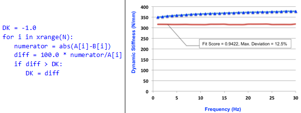
- The deviation metric for dynamic stiffness is simply the maximum deviation between two sets of dynamic stiffness curves, A(xk) and B(xk), expressed as a percentage.
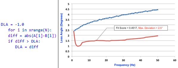
- The deviation metric for loss angle is the absolute value of the maximum absolute deviation between two sets of loss angle curves, A(xk) and B(xk), expressed in degrees
| Deviation Metric | Description |
|---|---|
| Dynamic Stiffness | Let A(xk), k=0…N-1 be a set of data points measured
experimentally. Let B(xk), k=0…N-1 be the corresponding set of data points from the analytical model. Let the
deviation metric for Dynamic Stiffness be DK. The
pseudo-code for calculating DK is:
 |
| Loss Angle | Let A(xk), k=0…N-1 be a set of data points measured
experimentally. Let B(xk), k=0…N-1 be the corresponding set of data points from the analytical model. Let the
deviation metric for Dynamic Stiffness be DLA.
The pseudocode for calculating DLA is:
 |