Steady State Response of Nonlinear Systems
Bushing measurements are typically provided in the frequency domain, and not in the time domain. Thus, for a given preload and frequency, the bushing is typically subjected to a sinusoidal input at a given frequency. The bushing response at steady state, for the given preload and frequency, is measured in terms of a dynamic stiffness (Kd ) and a loss angle ( ).
Dynamic stiffness is the frequency dependent ratio between a dynamic force and the resulting dynamic displacement. The force can have two components: a displacement-dependent or spring-force component and a velocity-dependent or damping-force component.
Loss angle is defined as the phase angle between the displacement and the force. This phase difference is caused by the presence of the damping forces. The ratio of the damping force to the spring force is often called the loss tangent. It is the tangent of the loss angle.
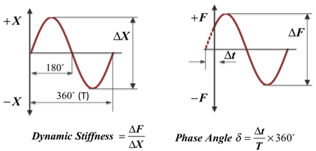
Figure 1.
Example of a Steady State Response of a Nonlinear Dynamic System
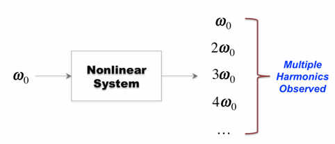
Figure 2.
The dynamic stiffness and phase angle are the response values of the system at the first harmonic ω0.
Dynamic Stiffness and Loss Angle of a Bushing Calculations
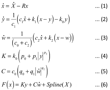
- Rubber Bushing Equations
-
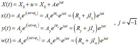
- The States
- For a sinusoidal input, at steady state and considering only the lowest
harmonic, the inputs and states for the bushing assume the
form:
(1) 
- The State Derivatives
- At steady state, the time derivatives of the states assume the form:
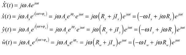
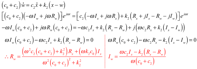
Figure 3. - Steady State Equations for a Rubber Bushing: Equation 1
- At steady state, equation (1) can be expressed:
(2) 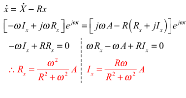
- Steady State Equations for a Rubber Bushing: Equation 2
- At steady state, equation (2) can be expressed:
(3) 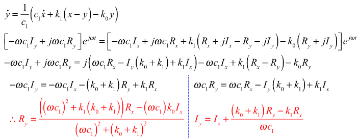
- Steady State Equations of a Rubber Bushing: Equation 3
- At steady state, equation (3) can be expressed:
(4) 
- Steady State Equations of a Rubber Bushing: Equations 4 and 5
- At steady state, equations 4 and 5 can be expressed:
(5) 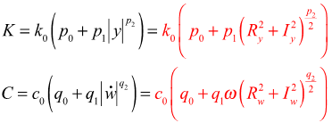
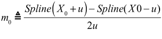
- Steady State Equations of Rubber Bushing: Equation 6
- In the physical test of the bushing, the bushing is provided an initial
preload deformation, X0,
and a dynamic oscillation, u, is
superposed on top of it. Therefore at steady state, the average slope
for an oscillation, u, about a
preload, X0,
is:
(6) 
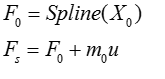
- The static response of the bushing for a dynamic oscillation,
u, is therefore:
(7) 
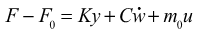
- Dynamic Stiffness is the ratio of the force change per oscillation cycle
divided by the displacement change. The static force
F0 at the
operating point cancels out during these calculations. We can
equivalently achieve this by just subtracting
F0 from the force,
therefore:
(8) 
- Substituting the expressions for y,
, X
and x, one gets:
(9) 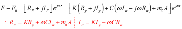
- Dynamic Stiffness and Loss Angle of a Bushing
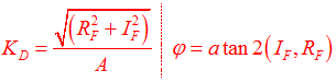
- You can compute the dynamic stiffness and loss angle as:
(10)