Create an Activate model that supplies a three-phase sine current into a Flux 2D model
of an Interior Permanent Magnet motor, and co-simulate the models.
The co-simulation process includes four basic steps:
Create a Flux model. For this tutorial, a Flux model of an IPM motor is provided for
you.
Generate the Flux coupling component required for Activate to read in the Flux model
data.
Create an Activate model and include the Flux block for reading in the Flux coupling
component.
A finished version of the models you build in the tutorials along with any files
required to complete the tutorials are available at this location:
<installation_directory>/tutorial_models/Flux_IPM.
Important: The co-simulation process requires the Flux files
(.FLU and .F2STA) to be located in the
same working directory. When naming the working directory, avoid spaces and special
characters as Flux cannot recognize them.
Overview of the Flux IPM Motor
The Flux model is a brushless, AC, Interior Permanent Magnet motor applicable for
electric vehicles.
The IPM motor is comprised of three main components:
Fixed part (stator) including yoke, slots, and windings
Air gap
Moveable rotor with embedded magnets
The IPM motor is driven with a three-phase sine current, running with kinematics type
Multiphysics position. The simulated motor performances are applied for computing torque,
phase current, speed and rotor position.
The inputs for the IPM motor are defined as multi-physical parameters and include:
I_1: Physical quantities: μr, Bs, Br
I_2 Electrical quantities: resistance, voltage, current
The outputs for the IPM motor are scalar I/O settings that retrieve values through the
sensors, formulas (torque) and parameters (position, speed, acceleration).
The circuit of the IPM motor is configured with a current source, coil conductor, resistor
and inductance.
Figure 1. Electrical circuit of IPM motor
Generating the Coupling Component in Flux
Load the Flux model and generate the coupling component with the required inputs,
outputs and parameters.
Launch Flux, and from your working directory, open the project,
IPM_motor_Multiphysics_positionF2STA.FLU.
The model loads and looks something like this:Figure 2. Cross-section view of IPM motor
From the Flux 2D toolbar, select Solving > Generate component for Activate coupling.
In the dialog, enter the following information for the component:
Enter the name for the component:
IPM_motor_Multiphysics_positionF2STA
Enter the path to your working directory:
<name_without_spaces>
Select the input (geometric I/O parameters) for the component:
I1, I2, I3
Select the output: PHASE_CURRENT_1,
PHASE_CURRENT_2,PHASE_CURRENT_3, TORQUE, SPEED_MOTOR and
POS_ROTOR
The dialog should look something like this:
Click OK.
The coupling component is saved to your working directory as IPM_motor_Multiphysics_position.F2STA.
Creating the Activate Model
Create a model to feed a three-phase sine current into the Flux model of the IPM
motor.
From Activate, create a new model and save it to your working directory as
IPM_motor_Multiphysics_positionF2STA.scm.
Alternatively, load the model:
<installation_directory>/tutorial_models/Flux_IPM/IPM_motor_Multiphysics_positionF2STA.scm and skip this section
of the tutorial.
From the Palette Browser, select Activate > CoSimulation, and drag one Flux block into your
diagram.
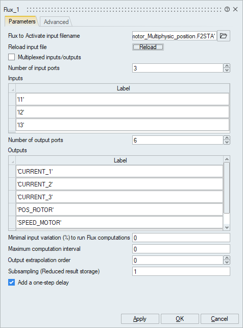
Double-click the Flux block. In the block dialog, for
Flux to Activate input filename, enter the path to
the coupling component you generated from Flux:
<working_directory>/
IPM_motor_Multiphysics_position.F2STA.F2STA.
Click OK.
The Flux block populates with the model data from the Flux coupling
component.
For the last three fields in the Flux block dialog, enter these values:
for Numerical memory (MB), enter 2721.
For Character memory, enter 200.
For Minimal input variation %, enter 10.
Click OK.
The Flux block dialog should look something like this:
In the diagram, add three SineWaveGenerator blocks to the left of the Flux
block and define them as follows:
Define
Sine Wave_1
Sine Wave_1
Sine Wave_3
Magnitude
200
200
200
Frequency (rad/s)
2 * pi * 80
2 * pi * 80
2 * pi * 80
Phase (rad)
45*pi/180
-2 * pi / 3+45*pi/180
-4 * pi / 3+45*pi/180
In the diagram, add four Scope blocks to the right of the Flux block, and
define them as follows:
Define
Scope 1
Scope 2
Scope 3
Scope 4
Block name
Currents
Rotor position
Rotor speed
Torque
Position
Number of inputs
3
2
1
1
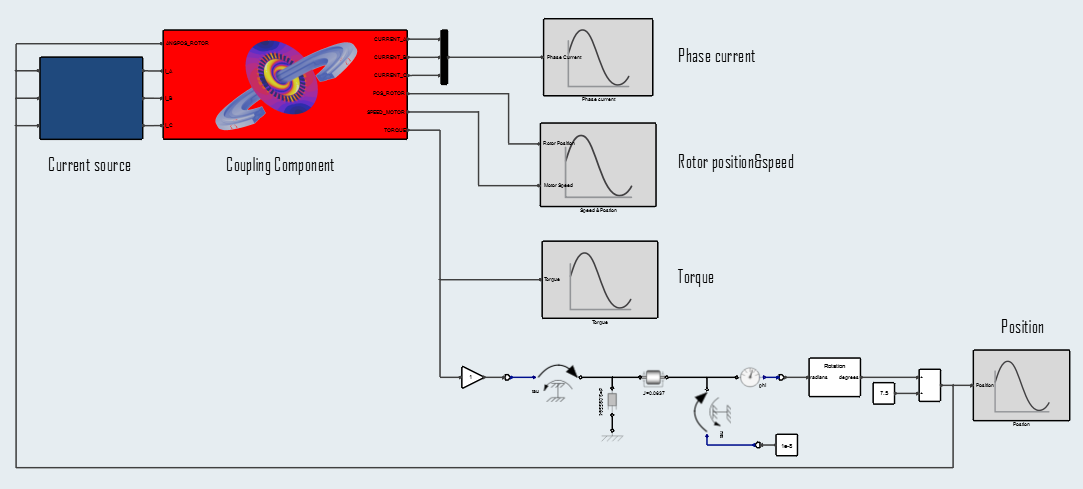
Assemble and connect the blocks as you see in the following figure, and save
the model.
Figure 3. Flux block assembled with inputs and outputs
The Activate model is complete and configured to supply the Flux model of the
IPM motor with three currents.
Co-Simulating the Activate and Flux Models
During co-simulation, the Activate model supplies a three-phase sine current into the
Flux model of the IPM motor. The simulation results show the performance of the IPM motor
including torque and losses at constant speed.
On the ribbon, hover over the Simulation tool group , and select Setup.
On the dialog that appears, select the Simulation Time
tab.
For Final Time, enter .0125. Keep the defaults for the
remaining fields.
Select the Solvers tab. For the solver, select
Forward Euler, and click OK. Keep the defaults for the remaining
fields.
On the ribbon, select Run.
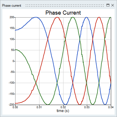
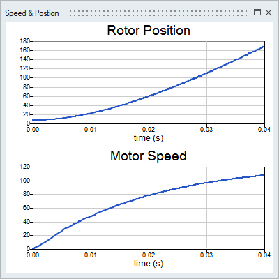
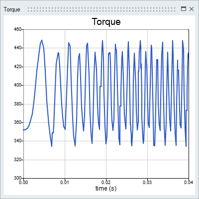
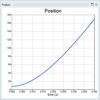
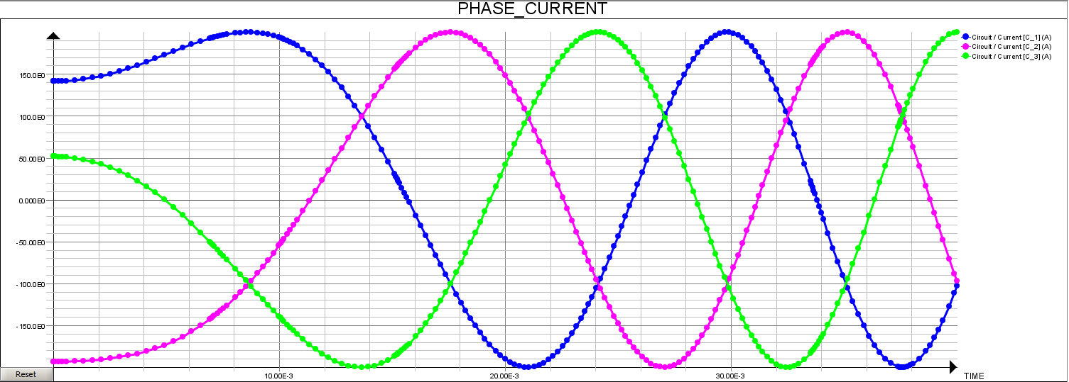
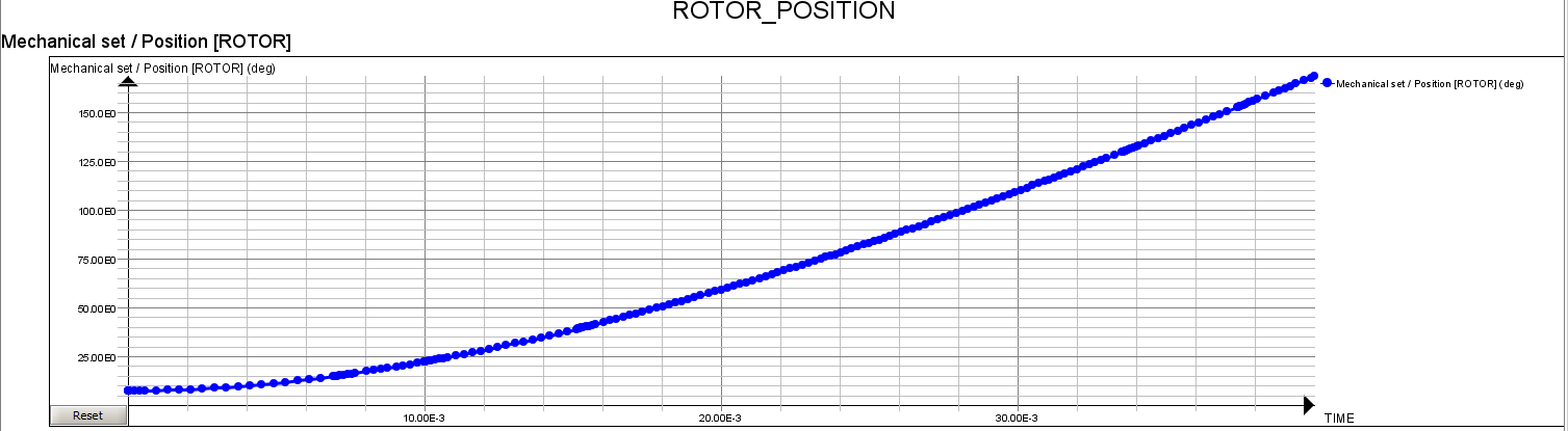
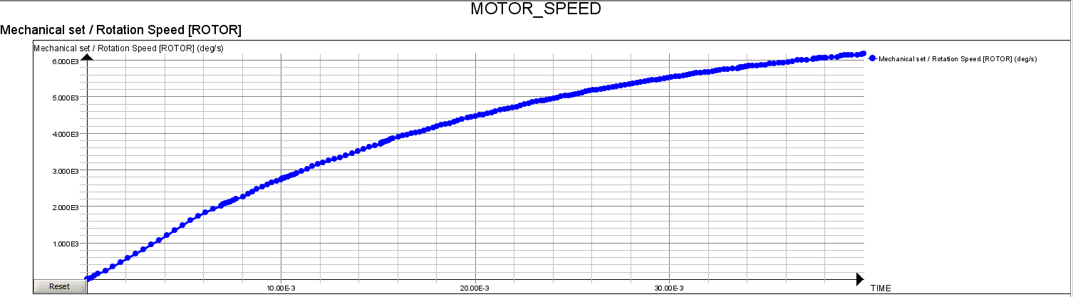
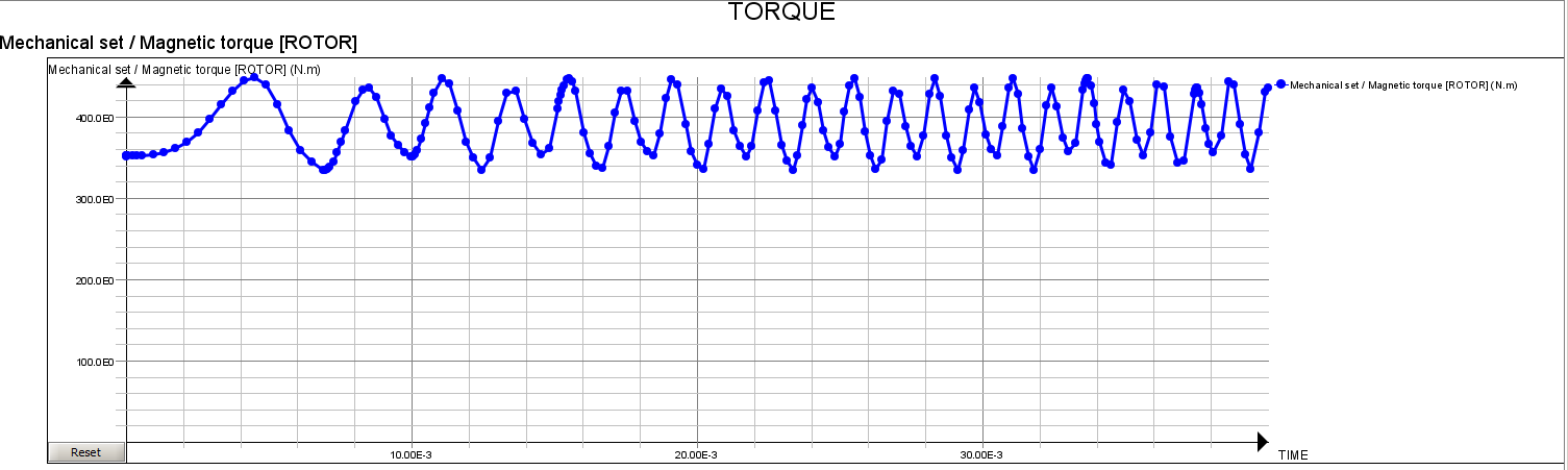
The simulation results show the currents fed into the motor and the
motor performance.Figure 4. Phase current (A), rotor position (deg), motor speed (deg/s), torque
(Nm) and position (deg)
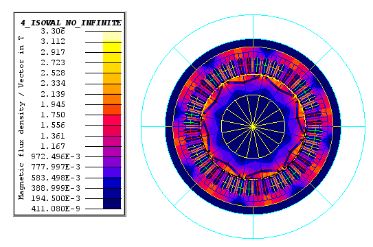
Flux post-processing results show density isovalues; phase current, rotor
position, motor speed, torque and position.
Figure 5. Flux density isovalues Figure 6. Phase current (A) Figure 7. Rotor position (deg) Figure 8. Motor speed (deg/s) Figure 9. Torque
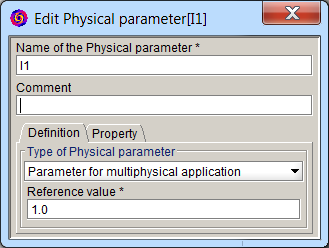
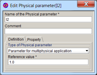
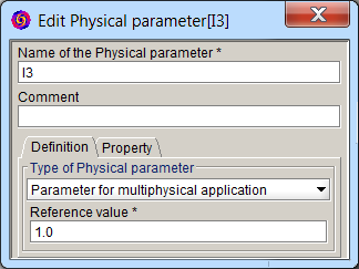
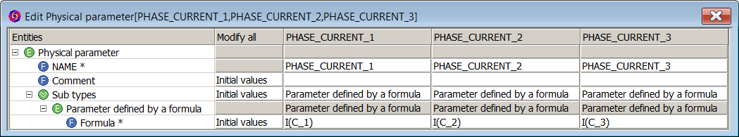
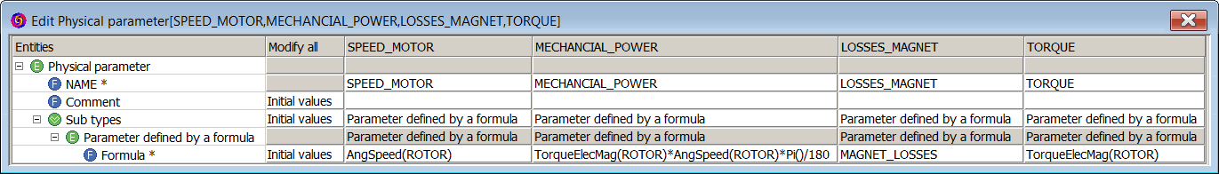
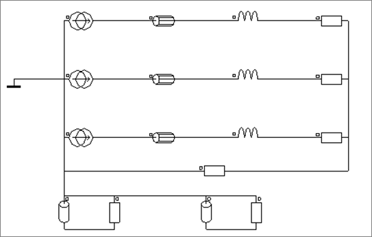 Figure 1. Electrical circuit of IPM motor
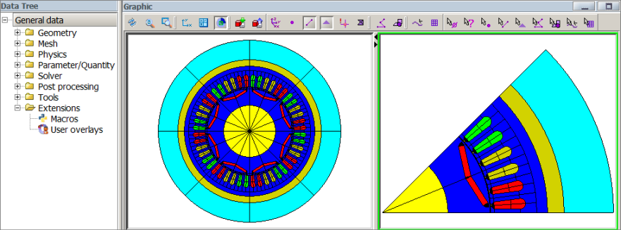 Figure 2. Cross-section view of IPM motor
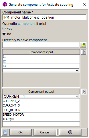
 , and select Setup
 .
.
 .
The simulation results show the currents fed into the motor and the motor performance.
.
The simulation results show the currents fed into the motor and the motor performance.