Example 7: FMCW Analysis
This case explains how to compute the FMCW spectrum of a simple geometry.
Step 1: Open newFASANT software and generate a new GTD-PO project selecting the option on the tab that appears when the 'File --> New' option of the menu bar is selected.
Step 2: Build the geometries. For this purpose the user can use all options available to construct geometries (see Geometry Menu). Generate a plane typing 'plane' on the command line panel, and introducing the following parameters when the command line ask for it:
- First corner of base [x y z] 6.0 10.0 0.0
- Box size [width depth] 5.0 2.0
- Height 1.0
Repeat the operation with the following parameters:
- First corner of base [x y z] -15.0 12.0 0.0
- Box size [width depth] 2.0 1.0
- Height 3.0
Repeat the operation with the following parameters:
- First corner of base [x y z] 8.0 -8.0 0.0
- Box size [width depth] 3.0 3.0
- Height 1.0
Repeat the operation with the following parameters:
- First corner of base [x y z] -10.0 -10.0 0.0
- Box size [width depth] 5.0 1.0
- Height 2.0
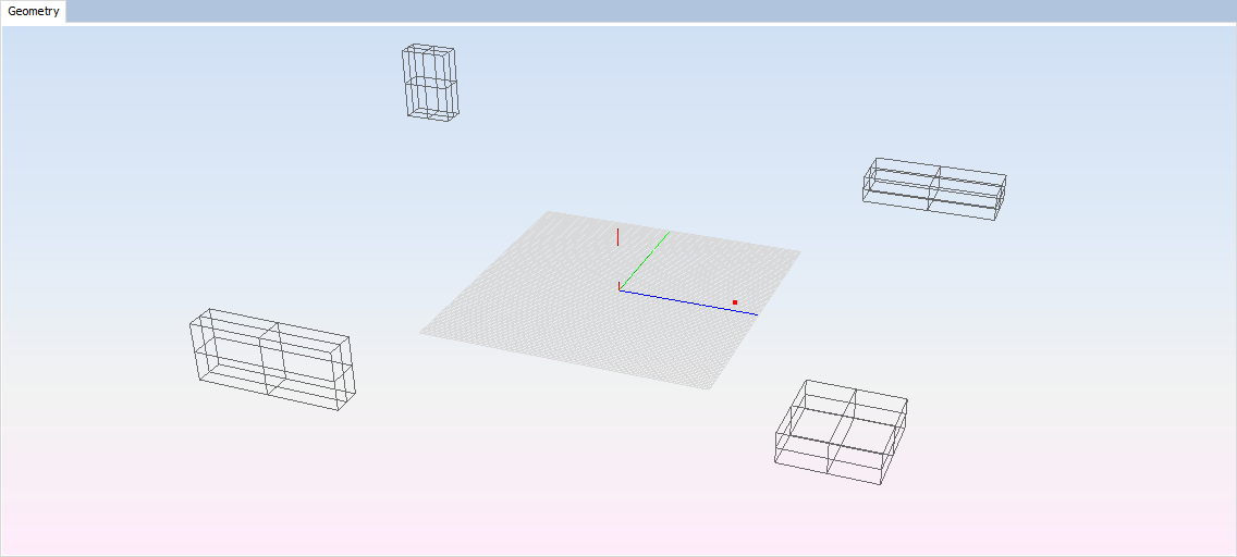
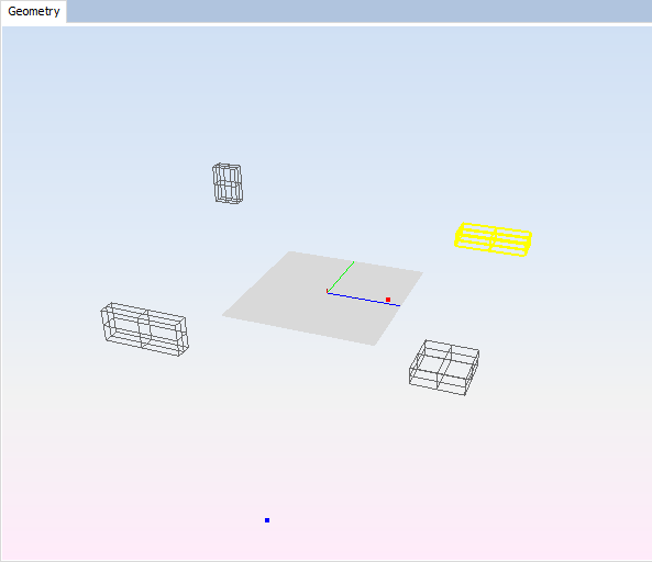
The following figure shows the created boxes:
Step 3: Set the simulation parameters using "Simulation --> Parameters" option on the menu bar.
Set ‘Method Type’ to GTD-PO, to analyze the scene classifying the object to analyze it with GTD or PO methods when corresponds.
Set ‘Simulation Type’ to ‘Doppler’ to analyze the scene considering Doppler effects.
Set the ‘Initial frequency’ to 24.05 and the ‘Units’ parameter to ‘GHz’.
Set ‘Number of bounces’ to 2 for the maximum number of rebounds of the rays.
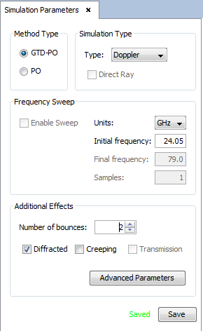
Figure 1. Simulation Parameters panel
NOTE: Selecting 'Doppler' option, "Output" menu is disabled on the menu bar and the observation will be forced to the same point that the source.
Step 4: Set the doppler parameters using "Simulation --> Doppler" option on the menu bar. With this option doppler effect will be added for the desired objects. Add the object selected in the next figure, selecting it and clicking on the “Add” button of the “Objects with doppler” panel.
Then set the parameters as the next figure shows, to add to the object a velocity of 10 m/s on the Y-Axis. Select "Enable/Disable FMCW" to obtain the analysis of 6 period of time with 0.01 seconds of duration. Then we analyze 6 periods of time with the movements on the object calculating the position of each moment with the duration of a period and the velocity.
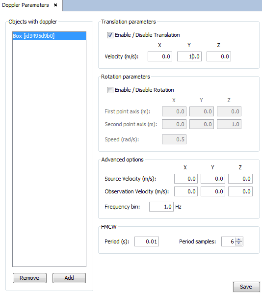
Figure 2. Dopler Parameters panel
NOTE: Selecting ‘FMCW’ options “RCS” menu is disabled and the RCS will be forced to monostatic.
Step 5: Set source parameters using "Source --> Source Parameters" on the menu bar. This option allows the user to locate the source defining the position by spherical or Cartesian coordinates. For this case select ‘Cartesian Coordinates’ and set the parameters as the following figure shows, to locate the source at the point 20.0,-6.0,1.0.
Set the ‘source size’ to 0.5 to optimal visualization of the source.
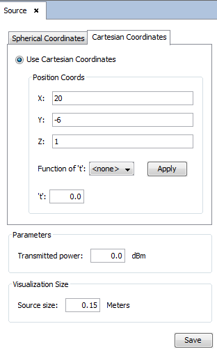
Figure 3. Source panel
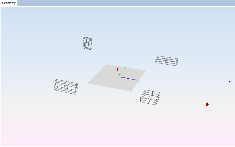
Clicking on ‘Save’ button the source appears on the main panel.
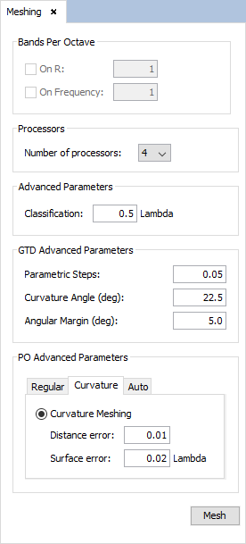
Then, the simulations for each period will be executed. When the execution has finished the result meshes can be opened with "Meshing --> Visualize an existing Mesh" option on the menu bar, and selecting the file from the directory of the selected step, frequency and period.
Step 7: Set calculate parameters using "Calculate --> Execute" option on the menu bar. The number of processors to be selected, to improve the efficiency on time, will be the number of the processors of the machine where the example will be executed.
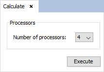
Then, the simulations for each period will be executed. When the simulations finish the results will be enabled to display it.
Step 8: Display the information about the field value with "Show Results --> Field --> View Cuts". The representation indicates the field component value on the observation point, in the case, the same point of the source, for a step, a frequency and period.
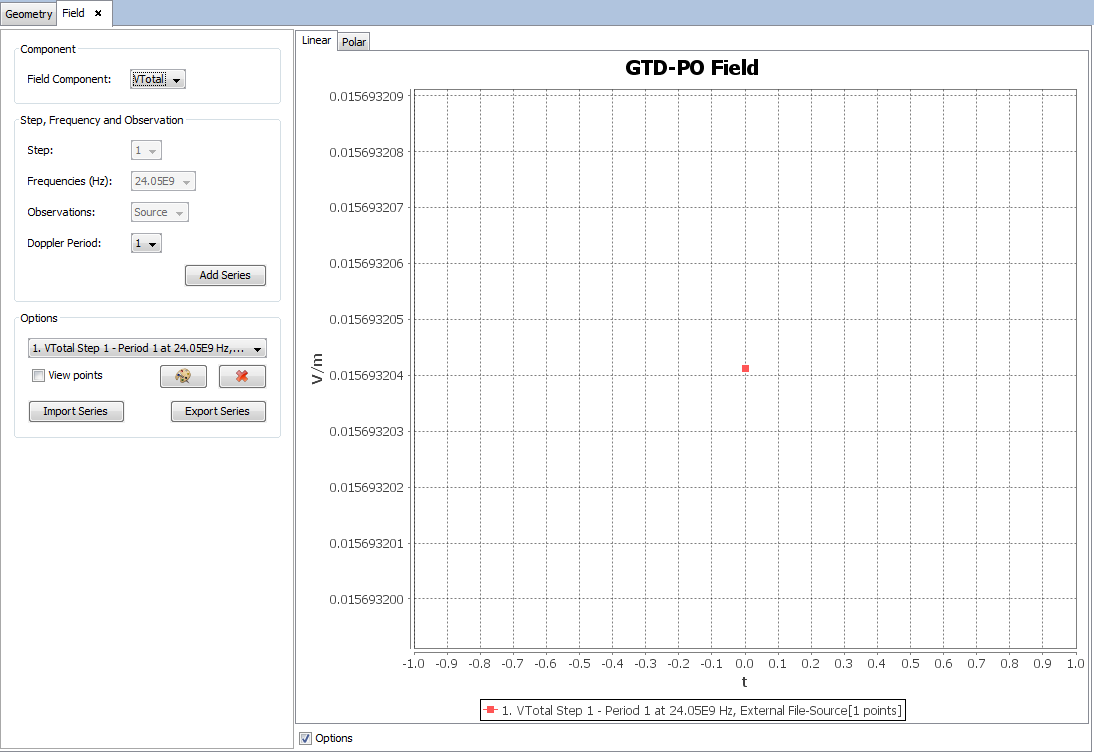
Selecting other field component, step, frequency or period and clicking on “Add Series” button adds other visualization of field.
Step 9: Display the information about the ray tracing with "Show Results --> Ray Tracing --> View Ray". The representation shows the rays for the selected step, period, frequency and source position. The rays can be filtered by effects and orders.
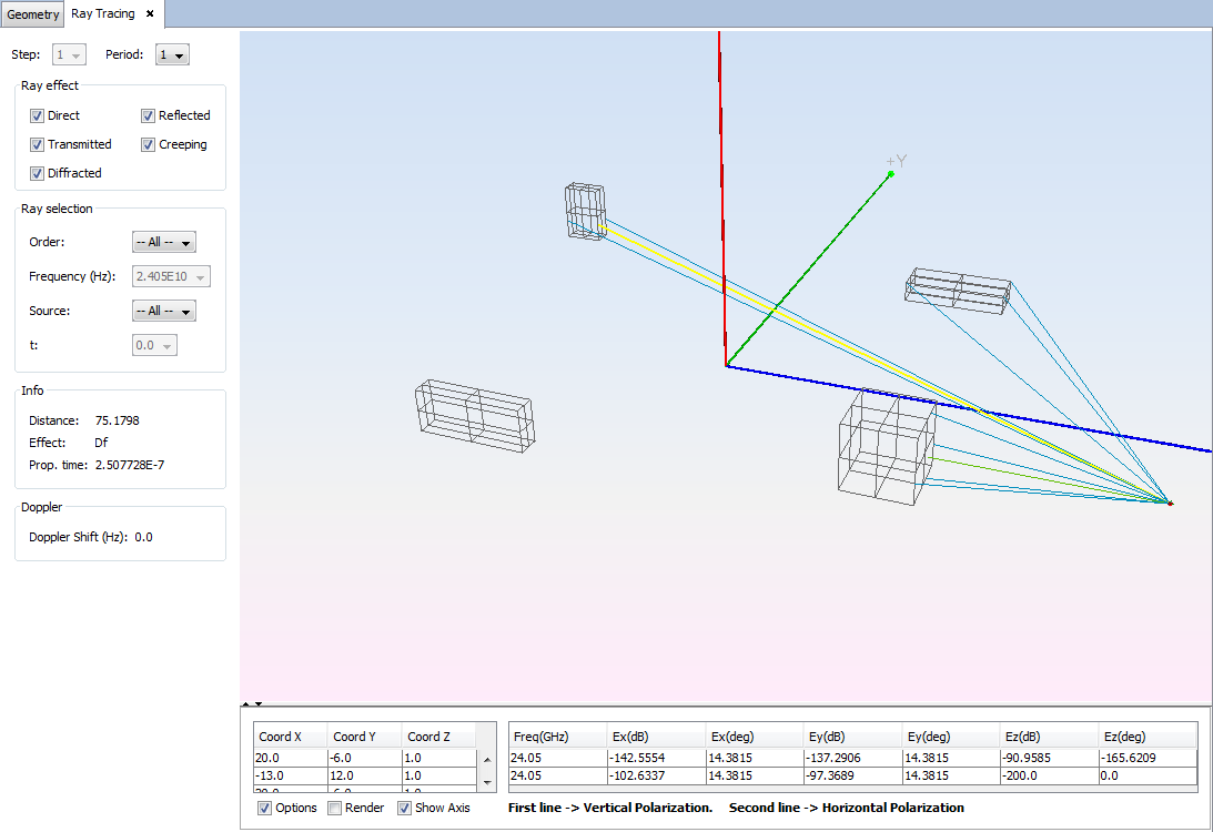
Selecting other step, frequency, period, position of the source or the orders and effects the visualization will be updated printing the rays that have the selected parameters. Selecting a ray into the panel, the information about it will be displayed on the tables at the bottom of the panel and on the ‘Info’ and ‘Doppler’ panels on the left panel.
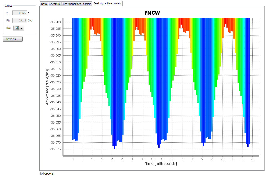
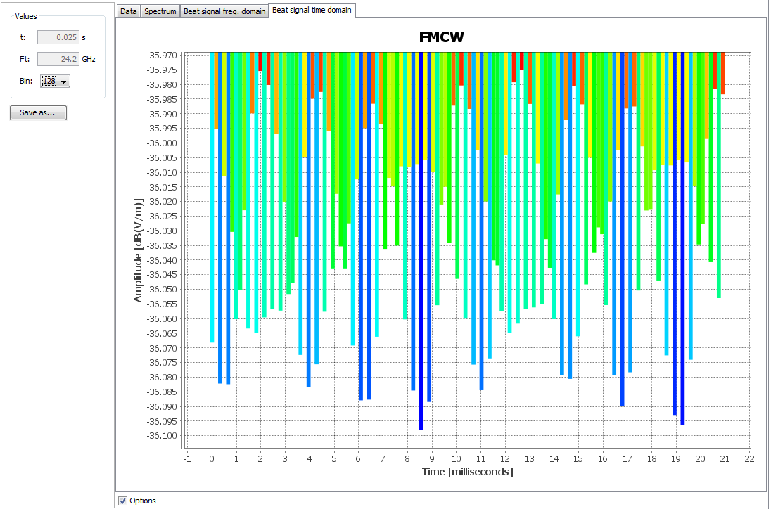
Step 10: Display the information about the FMCW spectrum with "Show Results --> Doppler --> FMCW". When this option is selected, appear a panel to set the parameters to calculate the FMCW Spectrum. These parameters are step, frequency, user function, maximum distance of the spectrum and the time to analyze. Press "Apply" button to visualize the frequency function. For this case, the parameters are correct to visualize the spectrum of the time 0.025 seconds.

Clicking on "View FMCW Spectrum" button the spectrum will be displayed.
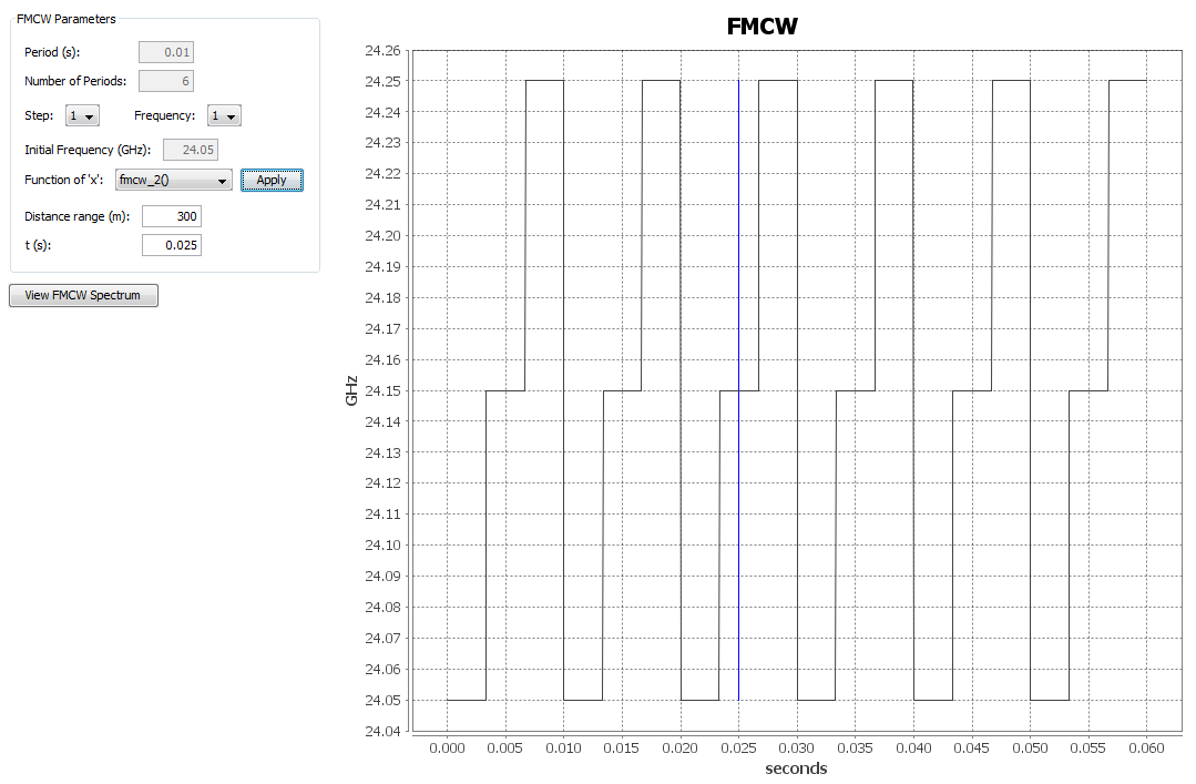
Step 12: To implement a function that defines the frequency in the time domain, open "Tools --> User Functions". Create a new file and programming the function using the global variables $x and $period. The $x variable defines the time. The $period defines the period and this variable is constant.
Example:
double fmcw_example(){
  // This function returns the frequency increment from time '$x'
  // Global parameters
  // $period period time in seconds.
  // $x time within the period.
  //
  // Note '$x' it is always less than '$period'
  //

  double x1 = 1./3 * $period;
  double x2 = 2./3 * $period;
  double x3 = $period;

  double y1 = 0.1;
  double y2 = 0.2;

  if($x < x1) {
    return y1/x1 * $x;
  } else if($x < x2) {
    return y1;
  } else {
    return y1 + ((y2-y1)/(x3-x2)) * ($x-x2);
  }
}
In the above example are defined three ranges, for each range defines a different function.
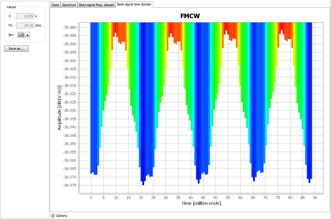
Save file and display the information about the FMCW spectrum with "Show Results --> Doppler --> FMCW". Select the function in the popup menu and press "Apply" button. The function will be displayed into the plot.

Introduce the time, for example t(s)=0.0225, to analyze and press "View FMCW Spectrum". Select the Bin into the popup menu to change the plots.