Calculate rural satellite coverage from a geostationary communications
satellite.
Model Type
The geometry is described by topography (elevation) and clutter/morpho (land
usage).
Figure 1. The topography (elevation) database used to determine the satellite
coverage.
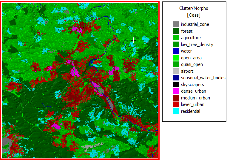
Figure 2. The clutter/morpho database used to determine the satellite
coverage.
Sites and Antennas
A single site, denoted Satellite 1, is located at a height of 36000 km and is
a geostationary satellite. The antenna has an EIRP1 of 90 dBm at a
carrier frequency of 2 GHz.
Tip: Click Project > Edit Project Parameter and click the Sites tab to view the
antenna settings.
Computational Method
The coverage is computed with the empirical two-ray model
(ETR) model. For pixels in
shadow areas, knife-edge diffraction is added for improved accuracy. Without this
addition, ETR would compute the path
loss to each pixel assuming that the direct ray and the ground-reflected ray exist,
which would be incorrect in shadow areas.
Tip: Click Project > Edit Project Parameter and click the Computation tab to change
the model.
Results
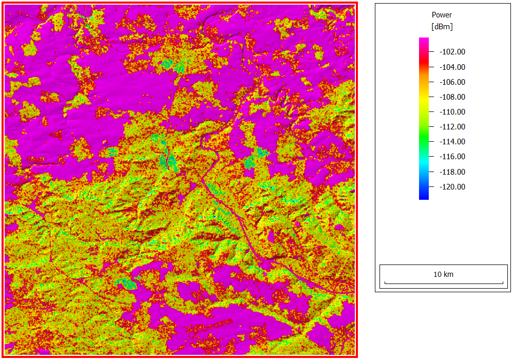
Propagation results are computed at a prediction height of 1.5 m and include power
coverage of each transmitting antenna and path loss. The power coverage (power
received by a hypothetical isotropic antenna) is shown in Figure 3.
Figure 3. Received power by a hypothetical isotropic antenna.
1 The actual transmitter power
in dBm plus antenna gain in the direction of interest in dB.