Strain-Life (E-N) Approach

Strain-life analysis is based on the fact that many critical locations such as notch roots have stress concentration, which will have obvious plastic deformation during the cyclic loading before fatigue failure. The elastic-plastic strain results are essential for performing strain-life analysis.

Neuber Correction

Neuber correction is the most popular practice to correct elastic analysis results into elastic-plastic results.

In order to derive the local stress from the nominal stress that is easier to obtain, the concentration factors are introduced such as the local stress concentration factor $K_{\sigma }$ , and the local strain concentration factor $K_{\epsilon }$ .

Where, $\sigma$ is the local stress, $\epsilon$ is the local strain, S is the nominal stress, and e is the nominal strain. If nominal stress and local stress are both elastic, the local stress concentration factor is equal to the local strain concentration factor. However, if the plastic strain is present, the relationship between $K_{\sigma }$ and $K_{\epsilon }$ no long holds. Thereafter, focusing on this situation, Neuber introduced a theoretically elastic stress concentration factor $K_t^{}$ defined as:

Substitute Equation 1 and Equation 2 into Equation 3 the theoretical stress concentration factor $K_t^{}$ can be rewritten as:

Through linear static analysis, the local stress instead of nominal stress is provided, which implies the effect of the geometry in Equation 4 is removed, thus you can set $K_t^{}$ as 1 and rewrite Equation 4 as:

Where, ${\sigma }_e$ , ${\epsilon }_e$ is locally elastic stress and locally elastic strain obtained from elastic analysis, $\sigma$ , $\epsilon$ the stress and strain at the presence of plastic strain. Both $\sigma$ and $\epsilon$ can be calculated from Eq.9 together with the equations for the cyclic stress-strain curve and hysteresis loop.

Cyclic Stress-Strain Curve

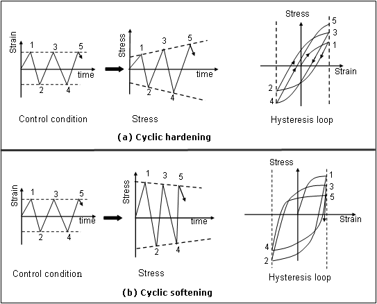
Which response will occur depends on its nature and initial condition of heat treatment. The figure below illustrates the effect of cyclic hardening and cyclic softening where the first two hysteresis loops of two different materials are plotted. In both cases, the strain is constrained to change in fixed range, while the stress is allowed to change arbitrarily. If the stress amplitude increases relative to the former cycle under fixed strain range, as shown in Material cyclic response (a), it is called cyclic hardening; otherwise, it is called cyclic softening (b).

Figure 1. Material cyclic response (a) Cyclic hardening; (b) Cyclic softening

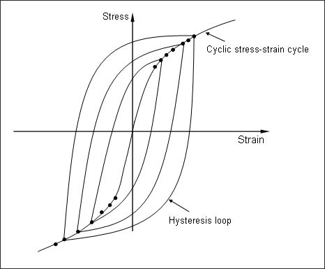
Cyclic response of material can also be described by specifying the stress amplitude and leaving strain unconstrained. If the strain amplitude increases relative to the former cycle under fixed stress range, it is called cyclic softening; otherwise, it is called cyclic hardening. In fact, the cyclic behavior of material will reach a steady state after a short time which generally occupies less than 10 percent of the material total life. Through specifying different strain amplitudes, a series of hysteresis loops at steady state can be obtained. By placing these hysteresis loops in one coordinate system, as shown in Figure 2, the line connecting all the vertices of these hysteresis loops determine cyclic stress-strain curve.

Figure 2. Definition of stable stress-strain curve

This can be expressed in the similar form with monotonic stress-strain curve as:

Hysteresis Loop Shape

Bauschinger observed that after the initial load had caused plastic strain, load reversal caused materials to exhibit anisotropic behavior. Based on experiment evidence, Massing put forward the hypothesis that a stress-strain hysteresis loop is geometrically similar to the cyclic stress strain curve, but with twice the magnitude. This implies that when the quantity $\left(\text{Δ}\epsilon ,\text{Δ}\sigma \right)$ is two times of $\left(\epsilon ,\sigma \right)$ , the stress-strain cycle will lie on the hysteresis loop. This can be expressed with formulas:

Expressing $\sigma$ in terms of $\text{Δ}\sigma$ , $\epsilon$ in terms of $\text{Δ}\epsilon$ , and substituting it into Equation 6, the hysteresis loop formula can be calculated as:

Almost a century ago, Basquin observed the linear relationship between stress and fatigue life in log scale when the stress is limited. He put forward the following fatigue formula controlled by stress:

Where, ${\sigma }_a$ is stress amplitude, $\sigma {\text{'}}_f$ fatigue strength coefficient, b fatigue strength exponent. Later in the 1950s, Coffin and Manson independently proposed that plastic strain may also be related with fatigue life by a simple power law:

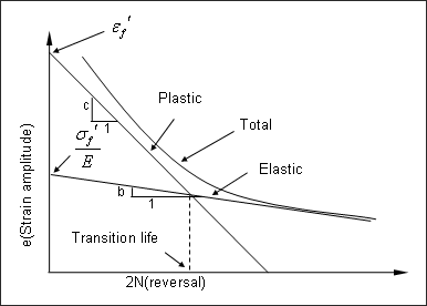
Where, ${\epsilon }_a^p$ is plastic strain amplitude, $\epsilon {\text{'}}_f$ fatigue ductility coefficient, fatigue ductility exponent. Morrow combined the work of Basquin, Coffin and Manson to consider both elastic strain and plastic strain contribution to the fatigue life. He found out that the total strain has more direct correlation with fatigue life. By applying Hooke Law, Basquin rule can be rewritten as:

Where, ${\epsilon }_a^e$ is elastic strain amplitude. Total strain amplitude, which is the sum of the elastic strain and plastic stain, therefore, can be described by applying Basquin formula and Coffin-Manson formula:

Where, ${\epsilon }_a$ is the total strain amplitude, the other variable is the same with above.

Figure 3. Strain-life curve in log scale