Set up and complete a solid profile extrusion analysis and post-process the data.
In this lesson you will learn about the Inspire Extrude interface and how to:
Import die geometry
Set up the solid profile extrusion analysis
Launch HyperXtrude solver
Post process the results
Given Data
This assumes a clean CAD model with solid components.
Data files are available in the tutorial_models folder in the
installation directory in Program Files\Altair\2021\InspireExtrudeMetal2021\tutorial_models\extrudemetal\tutorial-1\.
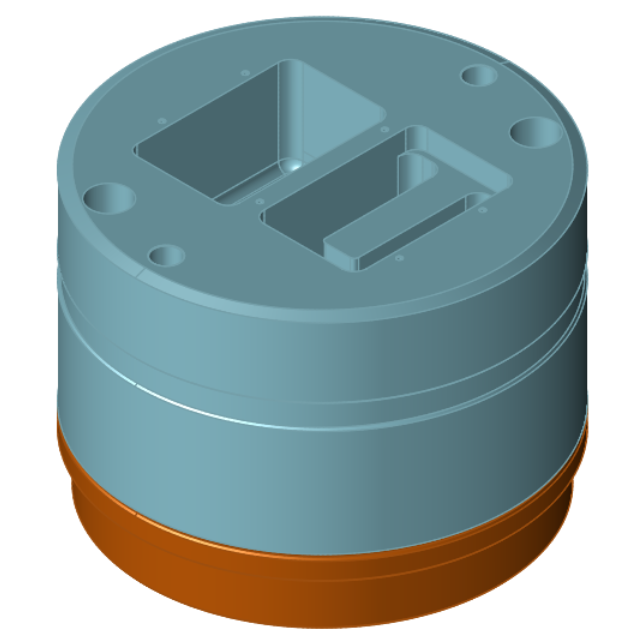
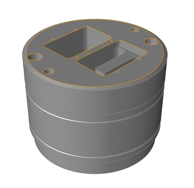
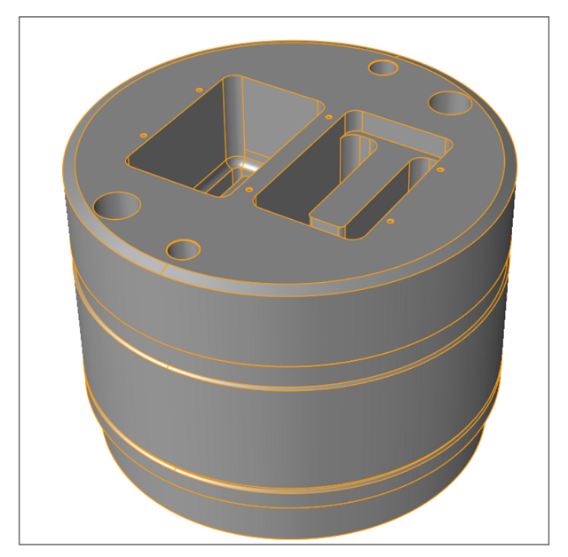
Model Details
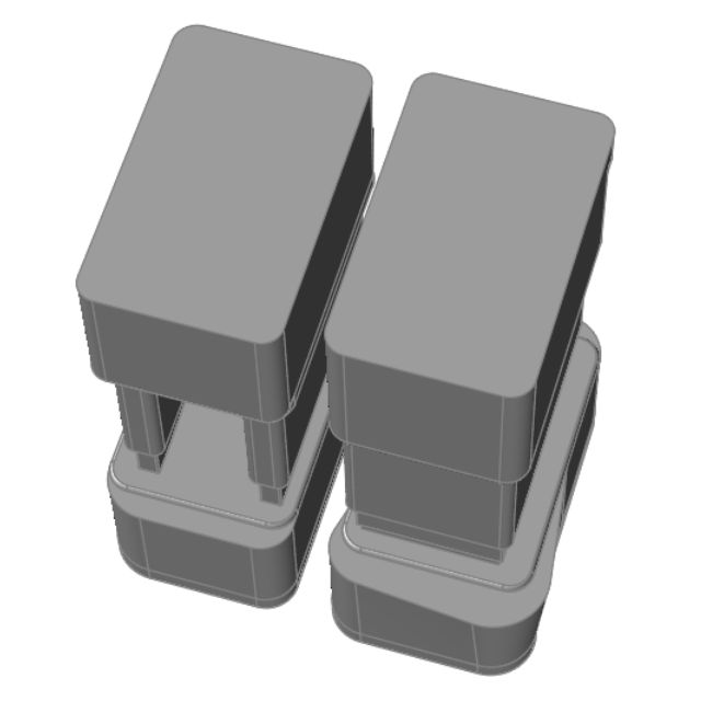
Model contains mandrel and die cap.
Two solid profiles are being extruded through this die
assembly.
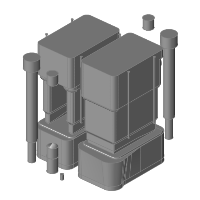
Import Die Solids
Click Start and search for Inspire Extrude, or double-click and launch Inspire Extrude from the shortcut on your desktop.
Import the die geometry, 3D_Die_Benchmark_2009.stp, either from the
File menu or by dragging the file into Inspire Extrude.
Click the Extrusion ribbon.
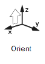
Click the Orient tool to position the model.
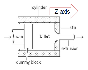
The die should be oriented such that the profile is coming out in the +Z
direction.
The center of the die face touching the billet is at X=0, Y=0, and Z=0
Select the die exit surface to orient the model.
Note: The die exit surface is where the profile exits the die.
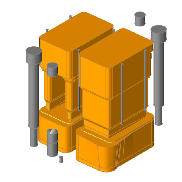
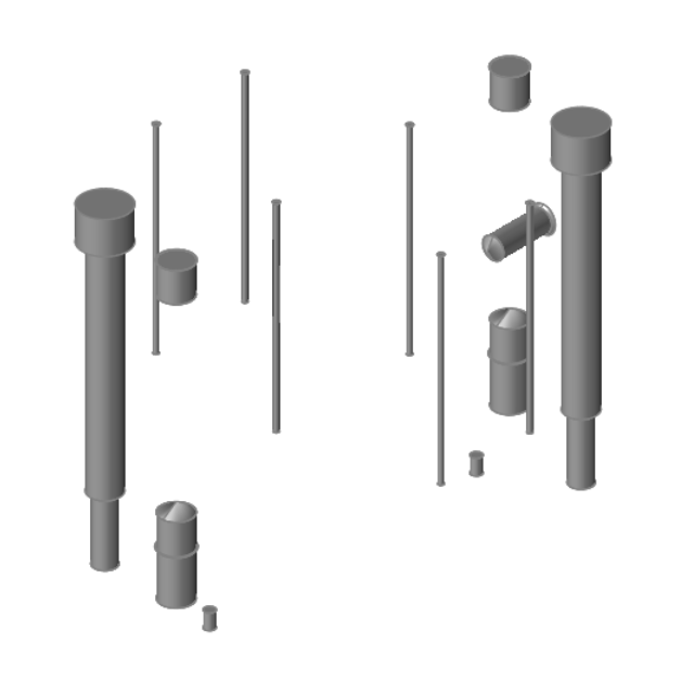
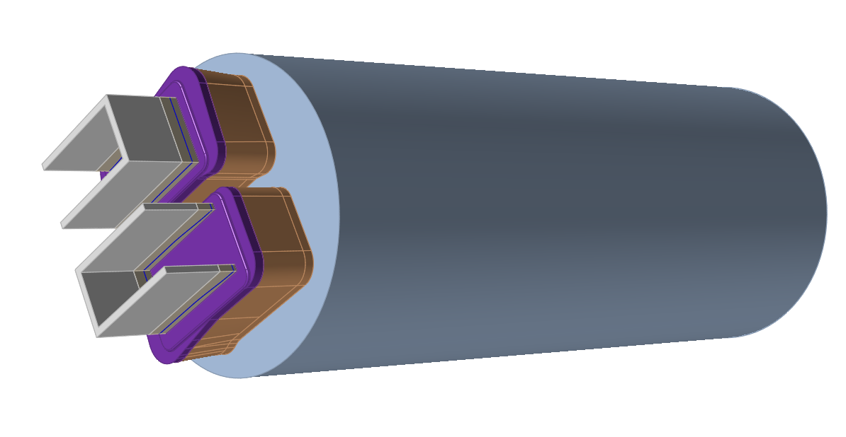
Extract Flow Volume
To simulate how aluminum deforms inside the die, we need to extract the volume
created by the die surfaces that come in contact with the aluminum.
Click the Flow Volume icon.
Click and drag to draw a rectangle around die geometry to select all die
solids as shown.
Release left mouse button to extract flow volume automatically.
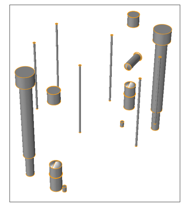
Refine Flow Volume
Select flow volume solids.
If there are multiple solids (as in this case), use
Ctrl for multiple selections.
Press H to hide selected flow volume solids.
Select solids to be deleted by drawing a rectangle around them, and press
Delete.
In this example, this will delete all screw pin holes and other solids
which do not belong to the flow region.
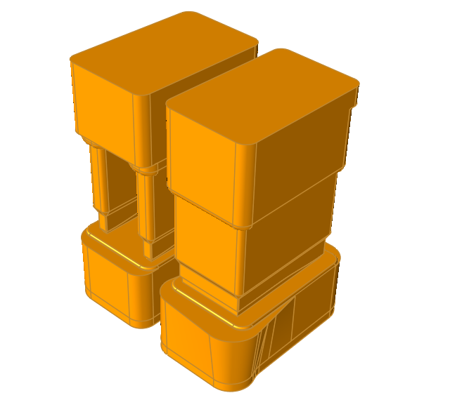
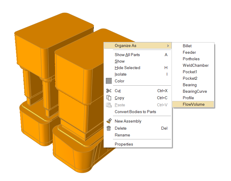
Combine Flow Volume
Hold CTRL and click on each flow solid as shown.
Right-click on either selected solid and click Organize As > FlowVolume.
The two separate Flow Volume pieces are now part of the same
FlowVolume piece.
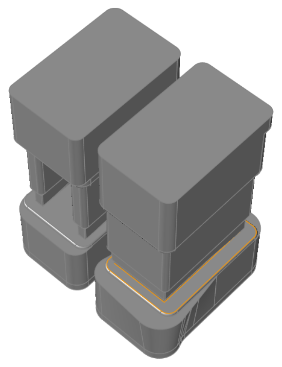
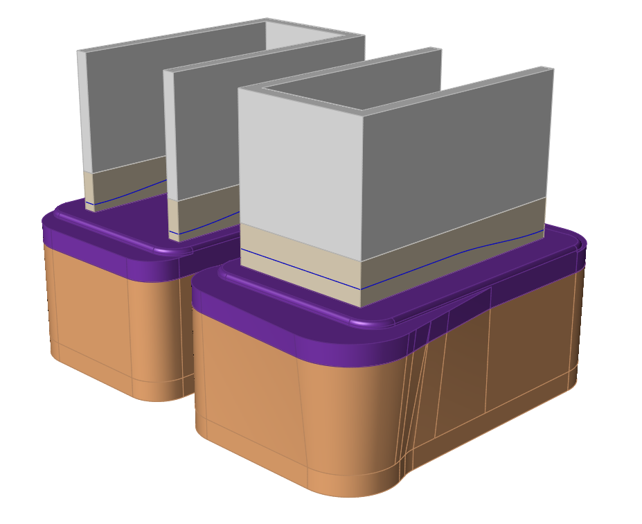
Extract Bearing Region
Zoom in to the region where bearing starts.
Click the Bearing icon.
Select the bearing start surface.
Program will automatically scan the geometry and discard the
relief region and create bearing and profile solids.
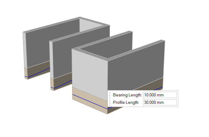
Note: Once the bearing is extracted,
you will be prompted to specify lengths for bearing and profile solids. You can keep
the default value and proceed. Profile region is 3 to 5 times the bearing
region.
Note: Profile is included in the model to capture how the profile
deflects.
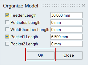
Organize Flow Volume
To better visulaize and interpret the results, we can organize solids into different
components using the manual cutting operation or by inputting predefined component lengths.
In this tutorial, we are going to use this latter option. This improves the ability to
create a good quality mesh with fewer elements.
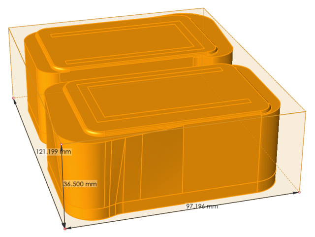
Check the flow volume length in the Z direction.
In our example it is 36.5mm. We will create the feeder and a small pocket
here.
Click the Organize volumes based on length icon.
In the small window that pops up, specify component lengths and click
OK.
Inspire Extrude will cut the flow volume length
based on the component lengths specified and organize them into their respective
components automatically.
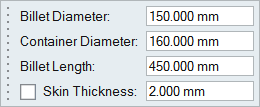
Create the Billet
We will specify the geometry to create the billet.
Click the Create Billet icon.
In the small window that pops up, specify billet and container dimensions and click
Enter.
Press Esc to exit this panel.
The billet is created to specified dimensions. The computation begins with upset billet, thus the billet is created with
upset length based on container diameter.
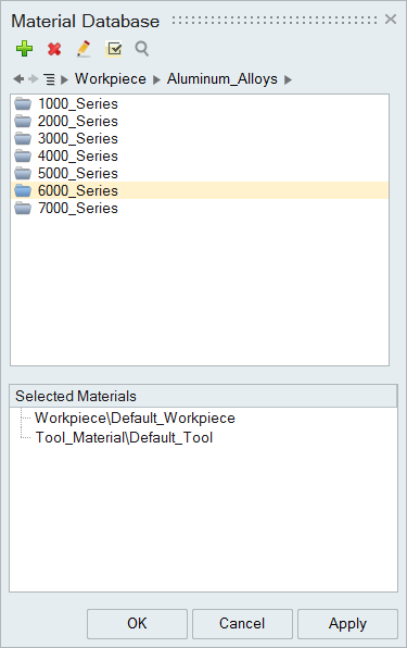
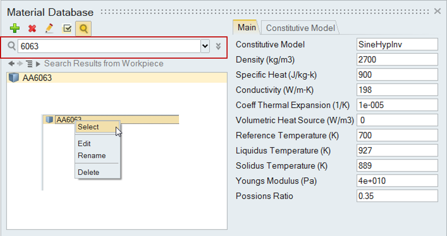
Select the Material
Click the Materials icon.
Select the Workpiece alloy Aluminum_Alloys > 6000_Series > AA6063
Note:
You can search directly for the material by clicking the search box
and typing the name of the alloy.
Right-click on the alloy name, and click Select.
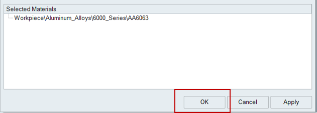
The chosen alloy is added to the Selected Materials pane.
Note: To deselect a material there, right-click and click
Deselect.
Click OK to close the Material Database.
Click File > Save As to save the model at the desired location.
Note: It is recommended that you always save the model file in a newly created
folder to avoid conflict with older/existing model files.
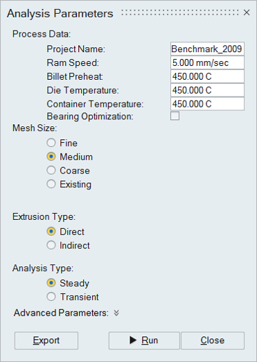
Specify Process Parameters and Simulate
Click the Submit job for analysis icon to run the
simulation.
In the Analysis Parameters window that pops up, enter
values as shown.
Click the Run button.
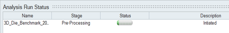
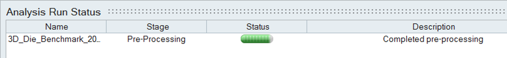
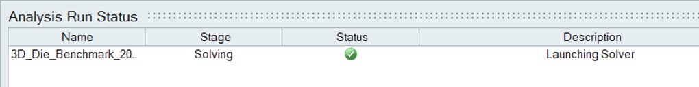
On successful launch of the run, you can monitor the status
of the simulation.
Status after submitting the job
Status after meshing is completed
Status when job is running in the solver
Review the OUT File
The goal of post-processing is to interpret the results generated by the solver and
apply it to understand the performance of the die and validate or improve the design.
Note: Results generated by the solver are in two key files
OUT file. This is an ASCII file that helps to verify the input data and
gives a quick overview of the result.
H3D file. This is a binary file with detailed results.
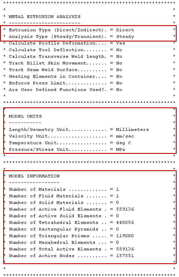
Verify the input data.
Check these sections of the *.out file:
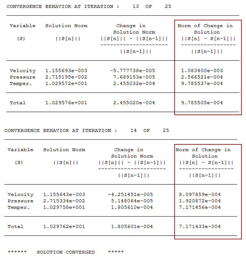
Solution Convergence
Mass Balance Table
Min/Max Velocity Table
Force Balance Table
Energy Balance Table
Solution Summary
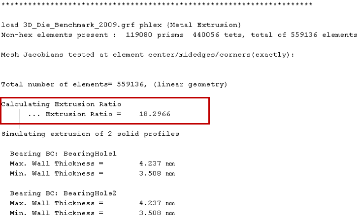
Verify the Extrusion Ratio is correct.
This is the ratio of the inlet area to the outlet area. This gives an overall
measure of how much the material deforms during extrusion.
If the value of the Extrusion Ratio is not correct, inspect the inflow and
outflow boundaries in the model to verify and correct them.
Check extruded profile Wall Thickness.
For this die, profile wall thickness varies from 3.5 mm to 4.2 mm.
Check the Analysis information.
Verify whether the Extrusion Type is Direct or Indirect and whether analysis
is Steady or Transient.
Review the unit system under the Model Units section.
Verify the Model Information including mesh size and type of elements
employed..
Tool material is denoted as Solid Material and extruded material as Fluid
Material.
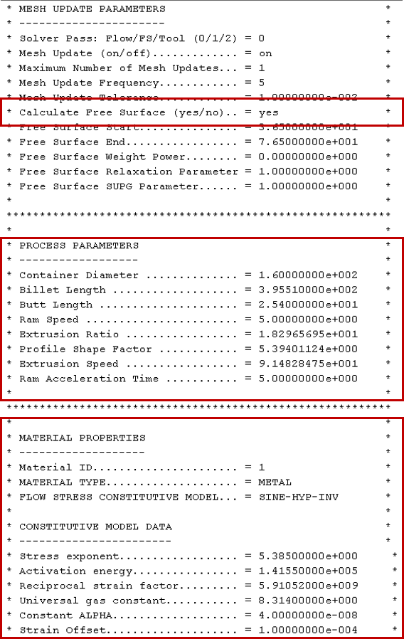
Verify the Mesh Update Parameters.
Check if the Free Surface calculation was performed and verify related
parameters such as Free Surface Start location.
Check the Process Parameters like Container Diameter, Billet Length, Extrusion
Speed, etc.
Review Material Properties.
Verify the voscosity model and associated consitutive model data.
Verify how the temperature dependency of viscosity is accounted.
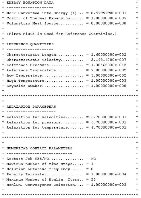
Examine Energy Equation Data.
Work converted into energy (%) accounts for viscous dissipation.
Check the reference quantities used in the analysis.
Verify different parameters used in the numerial solution.
Notice the relaxation parameters used in the solver.
Notice the convergence criterion used for the solution variables.
Check the Norm of Change in Solution.
Norm of Change may oscillate initially, but will decrease steadily after a few
initial iterations for all of the solution components (velocity, pressure, and
temperature).
The solution is considered "converged" if the value of Norm of Change in
Solution is less than tolerance (0.001) for all of the variables.
A slow convergence rate or oscillatory behavior indicates that the mesh is too
coarse.
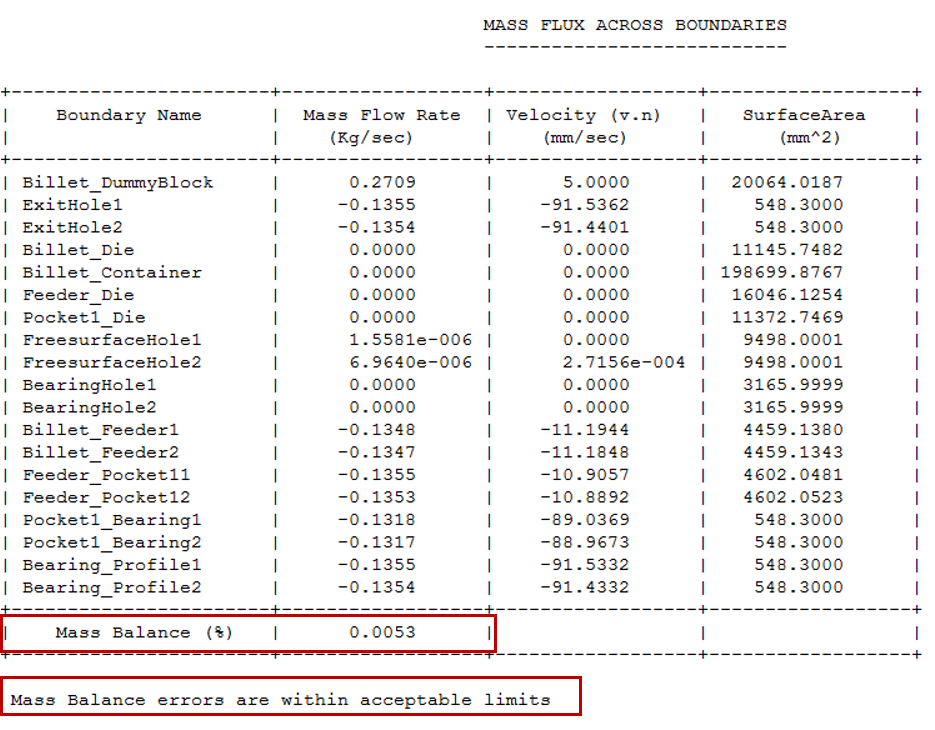
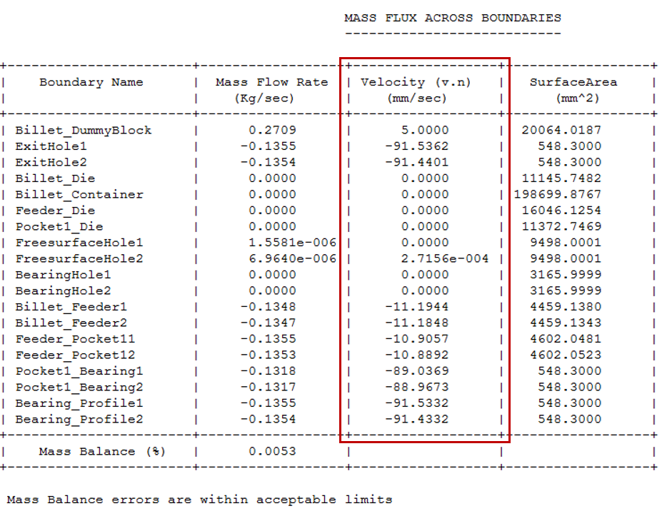
Verify that the Mass Balance is less than 1% to ensure conservation of
mass.
The Mass Flux table shows mass flow rate across each boundary,
A positive sign indicates material entering through the boundary, and a
negative sign indicates material leaving the boundary.
Check the average velocity of the material entering/leaving through each
boundary surface. If any of these checks fail, verify the boundary
conditions.
Velocity on solid walls must be close to zero.
Velocity on symmetry planes must be equal to zero.
Velocity on free surface boundaries must be small (at least a few orders of
magnitude less than the extrusion speed).
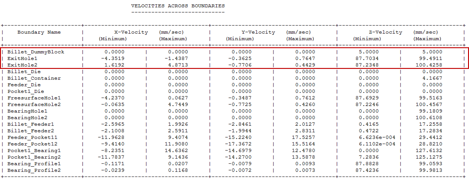
Verify that the profile exit velocity in the extrusion direction is
significantly higher than the velocity in the other directions.
Velocities in directions other than the extrusion direction indicate the
possibility of profile deflection.
Velocities at solid walls must be close to zero.
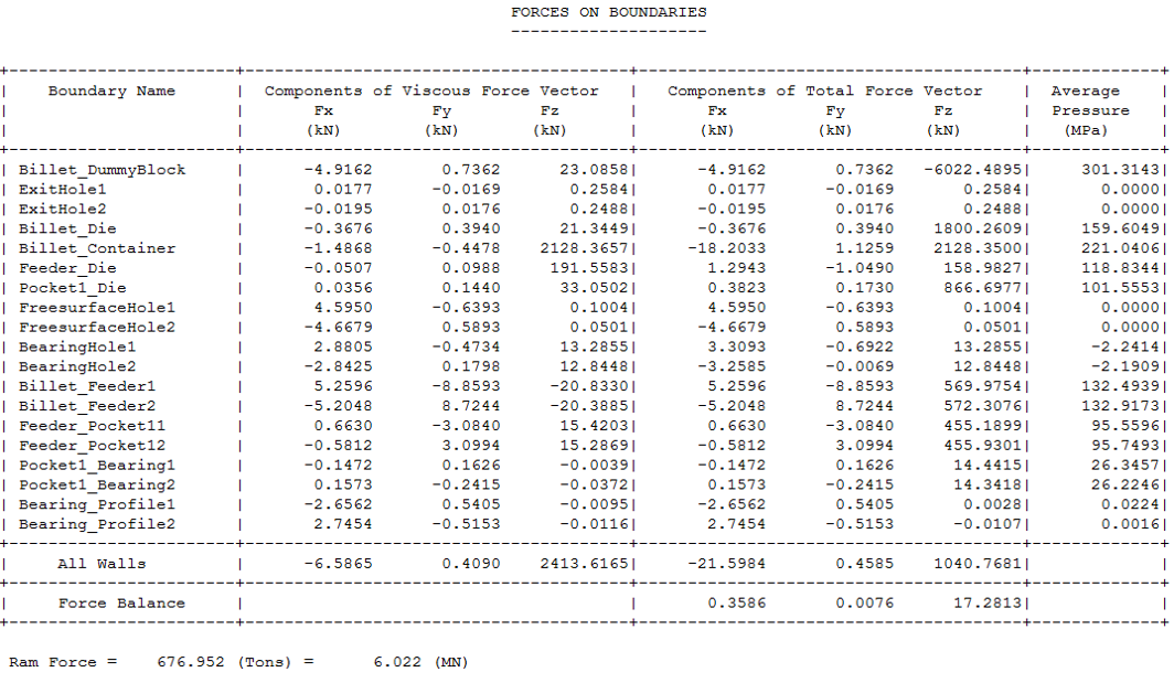
Review the Forces on Boundaries table.
A positive sign indicates force applied on a surface, and a negative sign
indicates response.
Verify that the force balance errors are within acceptable range
(~%5).
Verify that the average pressure at inlet is within the acceptable
range.
Verify the boundary conditions and material properties if any of these checks
fail.
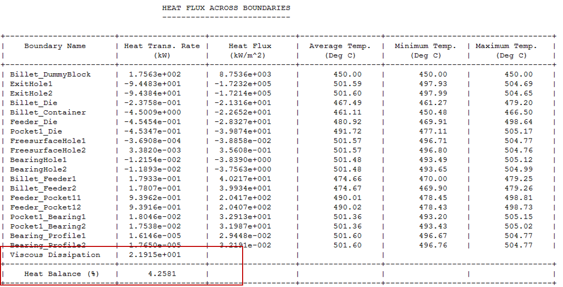
Review the Heat Flux Across Boundaries table.
A positive sign indicates energy input to the system, and a negative sign
indicates energy leaving through the boundary,
The table also contains average temperatures at each boundary surface.
Verify that the energy balance is less than 5%.
In this model, this is less than 5% and indicates a very good energy
balance.
Verify that average temperatures are within acceptable range.
Here, since all the walls are insulated, there is a small increase in
temperature due to viscous dissipation.
Verify the boundary conditions and material properties if either of these
checks fail.
Verify that the amount of heat generated during deformation is approximately
equal (within 5%) to the mechanical work.
This can be computed from the pressure on the inlet face, inlet velocity, area
of inlet face, and percent work converted to heat.
P = 264.73 MPa = 264.73 e+6
Pa
V = 5
mm/s = 0.005 m/s
A = 20064.03 mm^2 = 2.006e-2
m^2
%
conversion = 90%
Heat Generated = 264.73e+6 x 0.005 x
2.006e-2 x 0.9 = 23902.12W = 23.9 kW
Value of viscous dissipation from the Heat
Balance table = 21.88 kW
Difference is less than
5%
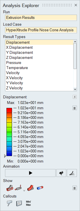
View Simulation Results
Use the Analysis Explorer to view the results.
This data provides a detailed understanding of how material deforms and flows during
extrusion. Using this data, we can detect flow imbalances at the die exit.
Understanding the material flow in die regions such as portholes and pockets helps
in redesigning to improve the performance of the die.
The pressure at the ram end provides the extrusion force required to push the
billet. This data also provides information on the resulting extrusion loads on
the die surfaces and can be used to predict tool deflection.
Understanding temperature distribution is the key to successful extrusion. Flow
stress of a material is a strong function of temperature and strain rate. In
addition, key material characteristics such as grain size depend on temperature.
Temperature data is used to determine where excessive heating occurs in the die due
to stress work. Temperature distribution in the profile region is used to determine
the surface quality and other material characteristics.
In the case of hollow profiles, the solver calculates seam weld location and
strength.
Click the various Result Types to change the analysis output.
Filter the results so that areas on the model with results greater than a
specified value are masked by clicking and dragging the arrow on the Results
Slider.
To change the legend color for the result type, click the
icon next to the Results Slider and select Legend
Colors.
To change the upper or lower bound for the Results Slider, click on the bound
and enter a new value. Click the reset button to
restore the default values.
Click the Play button to animate the selected result.
Click the icon to change the
speed of the animation.
Click the icon to open the
Scale by window. Generally, the scale of a
displacement is too small to see clearly, so autoscaling is enabled by
default.
Deselect the checkbox, and enter a different value to change the scaling
factor.
The icons under Show determine what is made visible in
the modeling window for the analysis.
Click the icon to hide the initial shape.
By default, the result is shown with the initial shape as a reference.
Click the icon to hide
the loads and supports.
By default, the result is shown with loads and supports.
Click the icon to show the deformed shape as a
reference.
Click the icon to hide the contours without blending.
Click the icon to reveal
additional options related to contours. Select
Interpolate during animation to animate the result
contour. Select Blended contours to toggle between
blended and non-blended contours.


 icon next to the Results Slider and select Legend
Colors.To change the upper or lower bound for the Results Slider, click on the bound and enter a new value. Click the reset button
icon next to the Results Slider and select Legend
Colors.To change the upper or lower bound for the Results Slider, click on the bound and enter a new value. Click the reset button to
restore the default values.
to
restore the default values. icon to change the
speed of the animation.
icon to change the
speed of the animation.
 icon to open the
Scale by window. Generally, the scale of a
displacement is too small to see clearly, so autoscaling is enabled by
default.
Deselect the checkbox, and enter a different value to change the scaling factor.
icon to open the
Scale by window. Generally, the scale of a
displacement is too small to see clearly, so autoscaling is enabled by
default.
Deselect the checkbox, and enter a different value to change the scaling factor.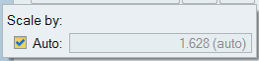
 icon to hide the initial shape.
By default, the result is shown with the initial shape as a reference.
icon to hide the initial shape.
By default, the result is shown with the initial shape as a reference. icon to hide
the loads and supports.
By default, the result is shown with loads and supports.
icon to hide
the loads and supports.
By default, the result is shown with loads and supports. icon to show the deformed shape as a
reference.
icon to show the deformed shape as a
reference.
 icon to hide the contours without blending.
Click the
icon to hide the contours without blending.
Click the