Manufacturing Solutions

HX-1201: Analysis of a Wire Coating Die

HX-1201: Analysis of a Wire Coating Die

Previous topic Next topic Expand/collapse all hidden text  

HX-1201: Analysis of a Wire Coating Die

Previous topic Next topic JavaScript is required for expanding text JavaScript is required for the print function  

Wire-coating dies are used to coat a metal wire with a thin layer of polymer. In this tutorial, you will learn to analyze a wire coating die using HyperXtrude. First, you will understand the manufacturing process to be simulated and the geometry of the configuration. This is essential to identify the computational domain and the process conditions. Then you will mesh the computational domain, set up the process conditions and launch HyperXtrude to solve.

hmtoggle_plus1greyFiles

The model files for this tutorial are located in the file mfs-1.zip in the subdirectory \hx\MetalExtrusion\HX_1201. See Accessing Model Files.

To work on this tutorial, it is recommended that you copy this folder to your local hard drive where you store your HyperXtrude data, for example, “C:\Users\HyperXtrude\” on a Windows machine. This will enable you to edit and modify these files without affecting the original data.  In addition, it is best to keep the data on a local disk attached to the machine to improve the I/O performance of the software.

Tutorial file - you will start from this file

- HX_1201.hm

Completed files provided for reference

- HX_1201_completed.hm


hmtoggle_plus1greyUnderstanding the Wire Coating Process

The coating of metal wires with a thin layer of polymer is an important process for cable and wire manufacturers. This is accomplished using a wire-coating die. The schematic of this process is shown in the following figure.  Polymer melt from the extruder is fed into the die and the metal wire is pulled in through the wire guide. The wire when exiting the die drags molten polymer along with it and it is cooled using a water bath (not shown in the figure).

HX_1201_01

A complete analysis of this process should include the metal wire (as the axial conduction along the wire is important) and the cooling of the coated wire after it exits the die. HyperXtrude can handle this process by doing a conjugate heat transfer analysis. To be conservative, a simpler version of the problem is considered and the domain studied is shown in following figure.

HX_1201_02

The problem at hand can be solved as an axisymmetric problem. However, to demonstrate the three-dimensional modeling capabilities of HyperXtrude, a 90-degree sector of the domain will be analyzed.

HX_1201_03


hmtoggle_plus1greyProcedure Used for Mesh Generation

It is beyond the scope of this tutorial to cover all aspects of mesh generation in HyperMesh. A brief sketch of the procedure is explained here.

HX_1201_04

The geometry to be meshed may be given to you in the form of a CAD file, which can be imported into HyperMesh. The CAD file may have more information than you actually need to generate the mesh and typically it may have few errors in the surface data. However, these inconsistencies can be handled easily in HyperMesh using the Geom Cleanup panel.  HyperMesh supports multiple CAD formats; of these, STEP and PART file formats come with the least errors. It is also easier to mesh starting from solids than from surfaces.

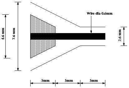
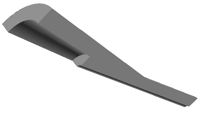
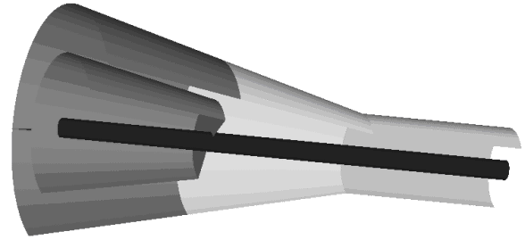
Meshing requires a clear strategy for successful completion. For instance, in this tutorial, you will model a sector of the wire-coating die. Meshing a longitudinal cross-section of the geometry and then spinning it by 90 degrees can generate this sector.  Assuming that you will proceed in this manner, the first step is to get the geometry data and form the 2-D surfaces.  The next step is to mesh the 2D surface using Automesh. Finally, a 3D mesh can be obtained by spinning the cross-section by 90-degrees using Spin. The 3D mesh should be checked using Check Elems and then renumbered using Renumber.

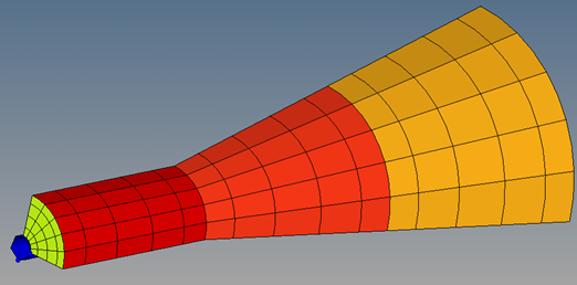
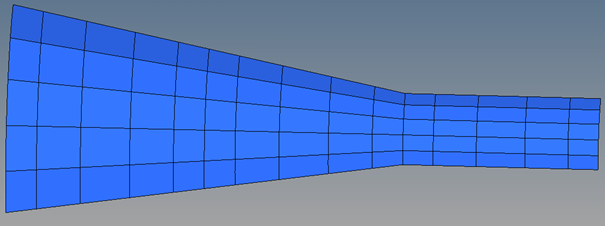
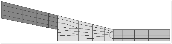
The 2D surfaces of interest are shown below. There are three surfaces from left to right: the feeder section, the tapering section and the coating section.

HX_1201_05

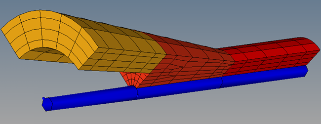
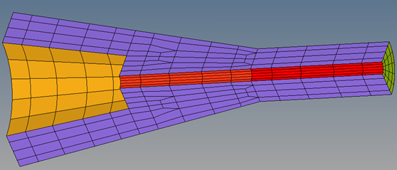
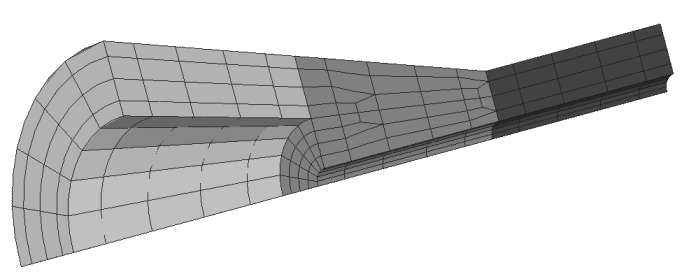
Automesh will automatically preserve the nodal consistency across the shared edges. The figure below shows the 2D mesh made of QUAD8 elements. Since the geometry of interest is a 90-degree sector, you need a higher order mesh (HEX20) to capture these curves accurately.

HX_1201_06

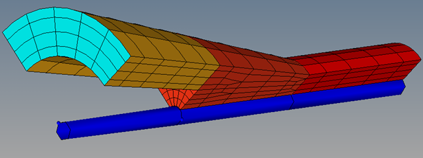
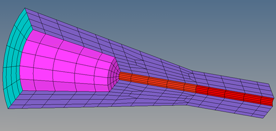
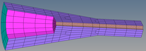
This 2D mesh is spun by 90-degrees about the Z-axis and with origin as the base-point.

HX_1201_07

It is important to do standard checks after meshing is complete. These can be done in the Check Elems panel.


hmtoggle_plus1greyStep 1: Launch HyperXtrude
1.Select Start Menu > All Programs > Altair Hyperworks > Manufacturing Solutions > HyperXtrude to launch the HyperXtrude User Interface. The User Profiles window appears with Manufacturing Solutions as the default application and HyperXtrude selected.

user_profile_pp

2.Select Polymer_Processing from the dropdown menu of HyperXtrude.
3.Click OK.


hmtoggle_plus1greyStep 2: Retrieve the model file
1.On the File menu, click Open.
2.Browse to the file HX_1201.hm.
3.Click Open to open the file.
4.Inspect the model.

hx_1201_model

The loaded model contains the completed mesh and its collectors, Feeder3D, Coating3D and Taper3D.


hmtoggle_plus1greyStep 3: Select units
1.On the Utility menu, click the Select Units macro.
2.Keep the Unit System as Metric and click OK.

model_units_metric

HyperXtrude allows you to work with a mixed set of units – that is, you can mix SI and British units. Selecting the model units should be the first step after loading the model.


hmtoggle_plus1greyStep 4: Select and assign materials
1.On the Utility menu, click Material Data.
2.In the dialog, expand the Polymers folder and select and load the material PVC_Generic.
3.Click Add. The entry moves into the Selected materials column.

HX_1151_10

4.Right-click PVC_Generic in the Selected material field and select Assign Material.

HX_1154_04

5.Select the Coating3D, Feeder3D, and Taper3D components and click Update.

HX_1201_11

Now you have loaded and assigned material data to the components. This completes this step and you can close the Material Data macro.

HX_1201_12


hmtoggle_plus1greyStep 5: Assign boundary conditions
1.On the Utility menu, click the Create/Edit BC macro. The first step is to edit the boundary data for Inflow.
2.Right-click BCs and select New.
3.Set the following options:

Name = Inlet

Type = Inflow

Material = PVC_Generic

Color = color of your choice

4.Click Create.
5.You will be prompted to edit the BC data. Set the following conditions:

Z-Velocity = 50 mm/s

Temperature =227 deg. C

6.Click Update.
7.Rotate the mesh and bring the inlet to a position where it can be seen.
8.Click Create Faces to assign BC face elements for this BC.
9.Select the inlet boundary elements by selecting one of the interior elements on the inlet face with the left mouse button. Selected faces will be highlighted.
10.Click proceed to create the BC faces.

HX_1201_14

11.Repeat steps 2-10 for Outflow. Use the image below to help determine where you should choose your element from. Data for Outflow is as follows:

Name = Outlet

Type = Outflow

Set traction, pressure, and heat flux values to zero. Check the Pressure checkbox to specify pressure at the outlet.

HX_1201_16

12.Repeat steps 2 -10 to set the following values for Symmetry:

Name = Symmetry

Type = SymmetryBC

HX_1201_18

13.Repeat steps 2 -10 to set the following values for outer surface BC Top Wall:

Name = Top Wall

Type = SolidWall

Friction Model = Stick

Heat Transfer Type = Temperature

Temperature = 127 deg C

Velocity = 0.00

HX_1201_19

14.Repeat steps 2 -10 to set the following values for the inner surface BC:

Name = InnerWalls

Type = SolidWall

Friction Model = Stick

Heat Transfer Type = Temperature

Temperature = 127 deg C

Velocity = 0.00

HX_1201_19b

15.Repeat steps 2 -10 to set the following values for the surface that is in contact with the wire:

Name = WireSurface

Type = SolidWall

Friction Model = Stick

Heat Transfer Type = Temperature

Temperature = 127 deg C

Velocity = 500 mm/s in Z; other two components are zero

HX_1201_19c

16.Click Update and close the dialog.

Now you have created and assigned all the boundary conditions required for the HyperXtrude run.


hmtoggle_plus1greyStep 6: Set process parameters
1.On the Utility menu, click Parameters.
2.On the Session tab, set the following parameters:

Set the Job/Model Name to HX_1201

Set the Job Description to WireCoatingDieAnalysis.

3.Click Update to save the data.

HX_1201_20

4.Inspect the data in the Polymer Processing tab. Make sure your data is identical to what is shown below.

HX_1201_21

5.Click on the User Commands tab and write the commands solve and exit under Footer Data.

You have successfully completed setting up data for the run.


hmtoggle_plus1greyStep 7: Save the model and launch the HyperXtrude solver
1.On the menu bar, click File > Save As and save the file as HX_1201_FINAL.hm at the desired location.
2.On the Utility menu, click Export/Launch Solver.
3.In the Project file name field, type HX_1201.grf and two files will generate with the names HX_1201.grf and HX_1201.tcl.
4.In the Project file name field, browse to locate the saved file location. Click Export. Two files will be generated with the names HX_1201_FINAL.grf and HX_1201_FINAL.hx .

HX_1201_23

5.Set the Launch solver field to No and submit the job on e-compute. Click on Launch to start the solver.

This concludes this tutorial.


Return to Polymer Processing Tutorials