This tutorial is used to quickly demonstrate how to prepare data for a transient analysis. In this tutorial, you will learn how to:
| • | Perform transient analysis |
| • | Solve for a moving boundary problem |
| • | Demonstrate the use of variable time step during transient analysis |
HyperXtrude can perform transient analysis of metal extrusion. It has two modes to perform these analyses: TransientFixedBoundary and TransientMovingBoundary. In this tutorial, you will use the TransientMovingBoundary option. In TransientFixedBoundary analysis, time-dependent behavior of the extrusion process is studied without actually moving the components of the model such as dummy block, etc. On the other hand, in TransientMovingBoundary analysis, movement of the dummy block and billet are simulated in the analysis.
The model files for this tutorial are located in the file mfs-1.zip in the subdirectory \hx\MetalExtrusion\HX_0302. See Accessing Model Files.
To work on this tutorial, it is recommended that you copy this folder to your local hard drive where you store your HyperXtrude data, for example, “C:\Users\HyperXtrude\” on a Windows machine. This will enable you to edit and modify these files without affecting the original data. In addition, it is best to keep the data on a local disk attached to the machine to improve the I/O performance of the software.
| • | Created Files (provided for reference) |
|
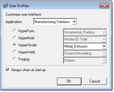
| 1. | Select Start Menu > All Programs > Altair HyperWorks > Manufacturing Solutions > HyperXtrude to launch the HyperXtrude user interface. The User Profiles dialog appears with Manufacturing Solutions as the default application. |
| 2. | Select HyperXtrude and Metal Extrusion. |
|
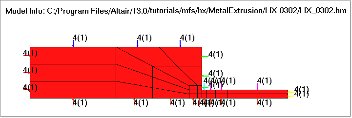
| 2. | Browse to and select the file HX_0302.hm. |
The imported data contains a 2D model with mesh, material properties, and boundary conditions. You will verify (or modify, if necessary) the existing model data.
|
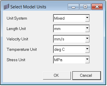
| 1. | On the Utility menu, click Set Model Units. |
Note: Measure dimensions of the model (ex: diameter of the billet) by pressing F4. Find the distance between any two nodes lying diagonally opposite to each other on the circumference of the billet. The numerical value of this distance (the diameter of the billet) gives you an idea about the unit system in which the model is created. Similarly you can verify the other dimensions of the model as well.
The current model is set up with meters as the length unit, m/s as the velocity unit, deg C for temperature and Mpa as the stress unit. Verify that the unit system is chosen as Mixed and the units are specified as shown in figure below.
The length unit of the current model is mm (Billet diameter is about 162).
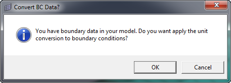
| 2. | Click OK. The Convert BC Data dialog is displayed. |
|
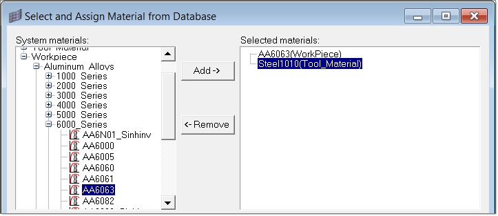
| 1. | In the Utility menu, click Material Database. |
| 2. | Verify that AA6063 is already selected as the material for workpiece (Billet). |
|
| 1. | In Utility menu, under BCs, click Create/Edit. The Create/Edit Altair HyperXtrude Analysis Boundary Conditions dialog displays. |
The BCs are already set up in the model with the following attributes:
| • | All interfaces with tool are specified as SolidWall, with no slip and no heat flux boundary condition. |
| • | BearingDie with Stick friction model and heat flux 0 W/m2. |
| • | BilletContainer with Stick friction model and heat flux 0 W/m2. |
| • | BilletDieface with Stick friction model and heat flux 0 W/m2. |
| • | BilletDummyBlock with XVelocity 0.002 m/s and a temperature of 500o C. |
| • | 2D models must be oriented with extrusion axis as X-axis. So XVelocity is set equal to Ram speed. |
| • | Outlet with standard traction boundary conditions with Pressure check box is selected. |
| • | ProfileSurface with heat flux 0 W/m2. |
| • | Symmetry with BC normal set to no |
| 2. | Click Close to close the dialog window. |
This model also illustrates how to build 2D models with HyperXtrude. This model is complete in all respects except for the process parameters.
|
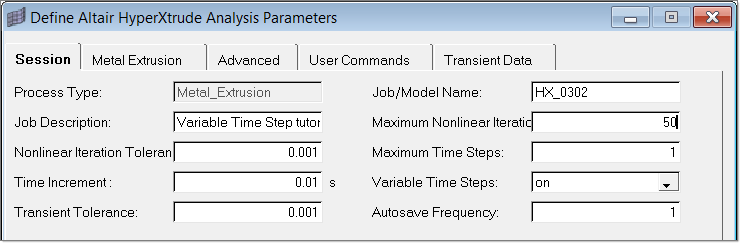
| 1. | In the Utility menu, click Parameters. The Define Altair HyperXtrude Analysis Parameters dialog displays. |
| 3. | In the Job Model/Name field, type HX_0302. This parameter is used to form the file name for the result files. Therefore, you should name it consistent with the operating system guidelines. |
| 4. | In the Job Description field, type Variable Time Step Tutorial. This parameter is used to print the string in the result window in the post-processor. |
| 5. | Set Variable Time Steps flag on. Turning this flag on will allow us to set up the time step data such as number of time steps (Num of Steps) and each time step size (Size) under Transient Data tab to be used during transient analysis. |
| 6. | Accept the default values for other fields and click Update. |
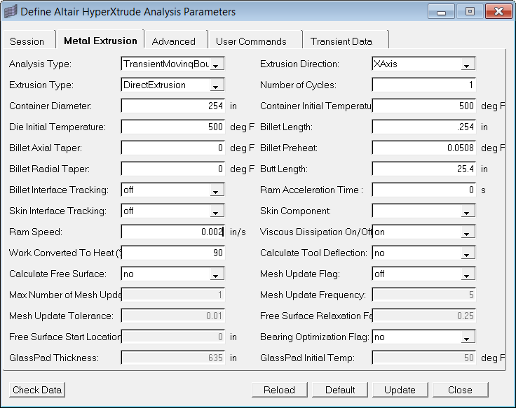
| 7. | Click the Metal Extrusion tab. |
| 8. | Set the Analysis Type field to TransientMovingBoundary. This parameter specifies that the analysis is transient and the billet is moving. Later specification is necessary to see the billet moving while being extruded in the simulation results. |
| 9. | Set the Extrusion Direction field to XAxis. 2-D models must be oriented with extrusion axis as X-axis. |
| 10. | Set the Billet Length field to 0.254m. |
| 11. | Set the Billet Preheat field to 480 deg C. |
| 12. | Set Butt Length = 0.0508 m. |
| 13. | Set Ram Speed = 0.002 m/s. |
Verify all other parameters, and if necessary, modify the values of the parameters to those shown in the figure.
| 15. | Click on the Transient Data tab. |
| 16. | Verify the data as shown in the image below and click on Update. |
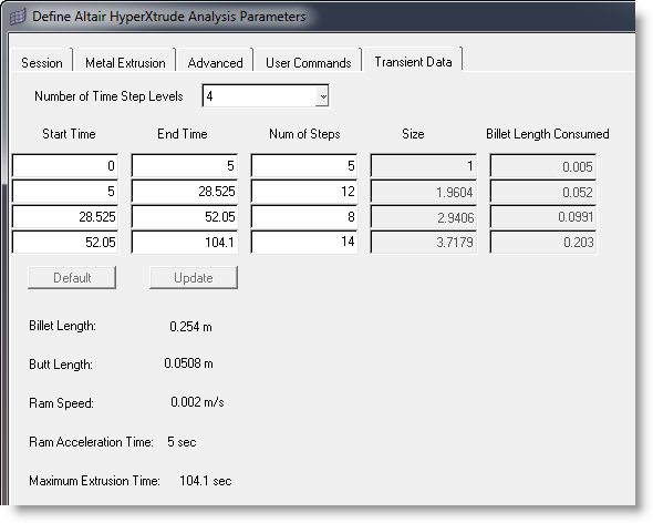
| 1. | By default, Number of Time Step Levels is set as 4 and the End Time for each time step level is also set. |
| 2. | If you want, you can modify Number of Time Step Levels, End Time and the number of time steps (Num of Steps) to be used for each level. |
For example, you can modify the default data as shown below.
Number of Time Step Levels = 3
End time = 5, Num of Steps = 5
End time = 20, Num of Steps = 5
End time = 100, Num of Steps = 16
| 3. | HyperXtrude is a fully implicit code; hence time steps can be large. However, you have to keep in mind how the boundary and other process data changes with time. For example, you should have at least few time steps for the first level (Start Time = 0 to End Time = Ram Acceleration Time) and so on. |
|
| 1. | Click File > Save As... and save the file as HX_0302_FINAL.hm. |
| 2. | In the Utility menu, click on Export Data Deck. |
| • | Model type = Two-Dimensional |
| • | Project file name = HX_0302_FINAL.hm in the directory of your choice |
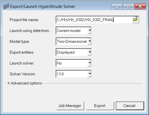
This writes input files for the solver (.hx and .grf data files).
|
When solving transient problems, it is advantageous to use the variable time step option and control the time step as function of time. This will ensure that you are using an optimal time step in each zone. This command allows you to specify at maximum five different time step levels. When you are using this option, HyperXtrude will ignore the parameters Maximum Time Steps and Time Increment and will use the data specified under Transient Data tab.
|
Return to Metal Extrusion Tutorials


