You can perform a bearing optimization using HyperXtrude and HyperStudy to ensure that the velocity of a profile is uniform. Bearing lines are used as design variables for the optimization with the objective to balance the flow at the exit.
HyperXtrude has a direct link with HyperStudy, which allows the design variables from HyperXtrude to be transferred to HyperStudy to perform the bearing optimization. To do this, you need a HyperStudy model that contains results to be optimized. The model must have the bearing lines that are defined. HyperStudy is launched from HyperXtrude and during the optimization, there is a constant communication between HyperXtrude, the solver, and HyperStudy.
Files
The model files for this tutorial are located in the file mfs-1.zip in the subdirectory \hx\MetalExtrusion\HX_0452. See Accessing Model Files.
To work on this tutorial, it is recommended that you copy this folder to your local hard drive where you store your HyperXtrude data, for example, “C:\Users\HyperXtrude\” on a windows machine. This will enable you to edit and modify these files without affecting the original data. In addition, it is best to keep the data on a local disk attached to the machine to improve the I/O performance of the software.
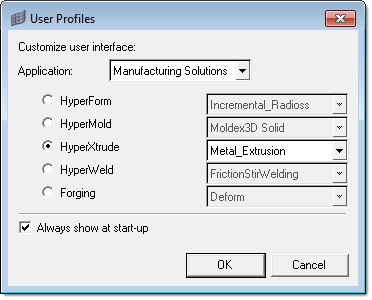
| 1. | Select Start Menu > All Programs > Altair HyperWorks > Manufacturing Solutions > HyperXtrude to launch the HyperXtrude user interface. The User Profiles dialog appears with Manufacturing Solutions as the default application. |
| 2. | Select HyperXtrude and Metal Extrusion. |
| 5. | Import the file HX_0452.hm into HyperXtrude. |
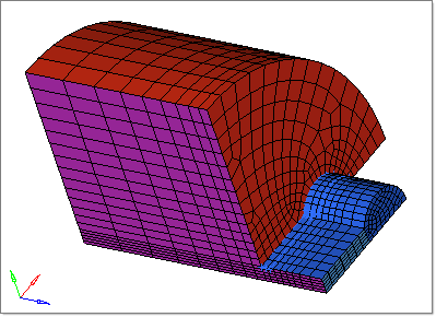
This is a simple "dog bone" model for bearing optimization. The velocity in the straight and curved sections needs to be uniform.
| • | For Billet_DummyBlock BC, RamSpeed of 5 mm/s and a temperature of 500 Cº are specified. |
| • | For Exit BC, standard traction boundary conditions are used. |
| • | All interfaces are specified at SolidWall, with slip and no heat flux boundary conditions. |
| • | Bearing profile is pre-defined. |
|
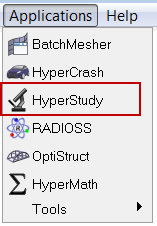
| 1. | From the Applications menu, click HyperStudy. |
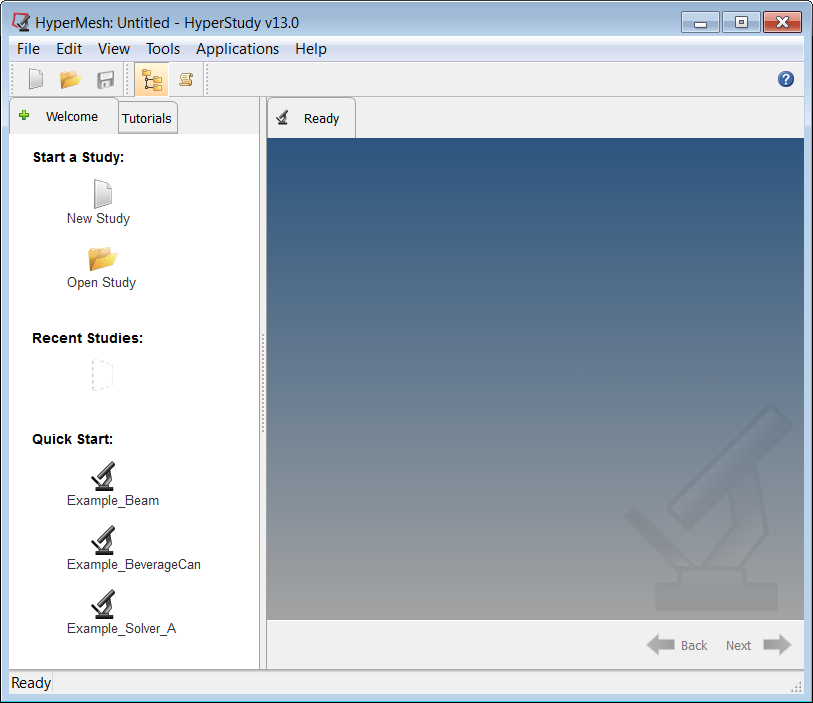
HyperStudy opens with the interface shown below:
|
| 1. | Click on File > New, or click New  in the toolbar. The HyperStudy - Add Study dialog appears. in the toolbar. The HyperStudy - Add Study dialog appears. |
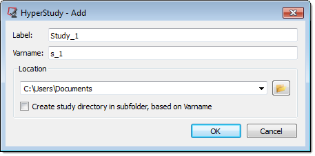
| 2. | Provide a Label: and a variable name (Varname:) for the study. |
| 3. | Browse to the location of the directory where the HyperMesh file is located. This location is where the files for the nominal run and the optimization will be written. |
| 4. | Click OK. A new study is created and the HyperStudy - Add Study dialog closes. |
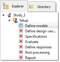
| 5. | Click Next twice to continue on to the Define models step, or click Define models in the study Explorer. |
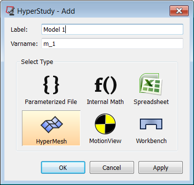
| 6. | Click Add Model  . The HyperStudy - Add dialog appears. . The HyperStudy - Add dialog appears. |
| 7. | Provide a Label: and a variable name (Varname:), and then select HyperMesh as the model type. |
| 8. | Click OK to add a new HyperMesh model to the Define models table, and to close the HyperStudy - Add dialog. |
| 9. | Click Import Variables  to import the design variables from the model. The Model Parameters dialog appears. The dialog contains the bearing lines in HyperXtrude on the left. These bearing lines can be added to HyperStudy after specifying the upper and lower bounds for the optimization. to import the design variables from the model. The Model Parameters dialog appears. The dialog contains the bearing lines in HyperXtrude on the left. These bearing lines can be added to HyperStudy after specifying the upper and lower bounds for the optimization. |
| 10. | In the Lower bound: field, enter 0.0. |
| 11. | In the Upper bound: field, enter 25.4. |
| 12. | Activate both Apply to all selected items checkboxes. |
| 13. | Expand Bearing under HyperMesh Model Parameters, and select all of the bearing lines. |
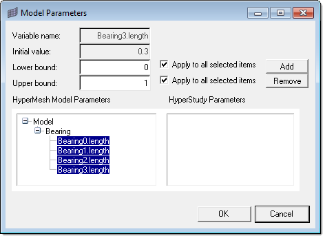
| 14. | Click Add to add the bearing lengths as HyperStudy parameters. |
| 15. | Click OK to close the Model Parameters dialog. The bearing lengths from HyperXturde are added as design variables in HyperStudy. |
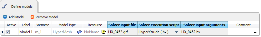
| 16. | In the Solver input file column for Model_1, enter HX_0452.grf. |
| 17. | Click on Solver execution script > HyperXtude (hx). |
| 18. | In the Solver input arguments field, enter HX_0452.hx. |
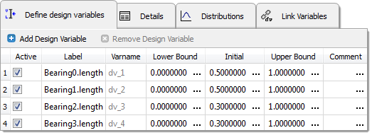
| 19. | Click Next to continue on to the Define design variables step. |
| 20. | Review the design variables. |
| 21. | Click Next to continue on to the Specifications step. |
| 22. | In the Specifications table, make sure the Mode is set to Nominal Run and then click Apply. |
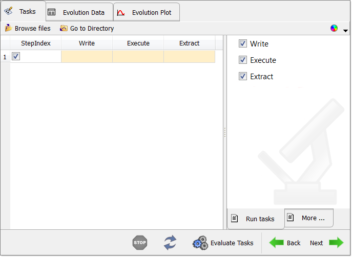
| 23. | Click Next to continue on to the Evaluate step. |
| 24. | Make sure the task manager settings Write, Execute, and Extract are all checked. This will create a folder with a name nom_run and a subfolder m_1 inside it under the specified directory (chosen above). It also writes the input files for the solver inside m_1. |
| 26. | Click Next to continue on to the Define responses step, where you will export the HyperXtude data files and run the analysis in batch mode. |
A nominal run with the initial bearing profile will be performed and the output files will be written inside the folder mentioned above in step 24.
|
| 1. | Load the nominal result file HX_0452.h3d into HyperView. |
| 2. | In HyperView, turn off the components other than the Profile3D component. |
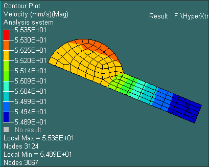
| 3. | Click Contour icon  and set the Result type as Velocity and click Apply. This will display velocity contours from the nominal run (i.e. without design variables being applied). If the display is different, click Edit Legend to adjust the legend to the values shown in the image. and set the Result type as Velocity and click Apply. This will display velocity contours from the nominal run (i.e. without design variables being applied). If the display is different, click Edit Legend to adjust the legend to the values shown in the image. |
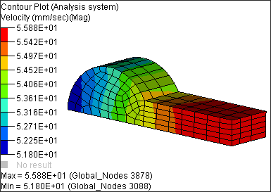
Velocity contour at the exit from the Nominal run
| 4. | Click Section Cut  and create a section cut in the +ve Z direction. Select a node and click apply. and create a section cut in the +ve Z direction. Select a node and click apply. |
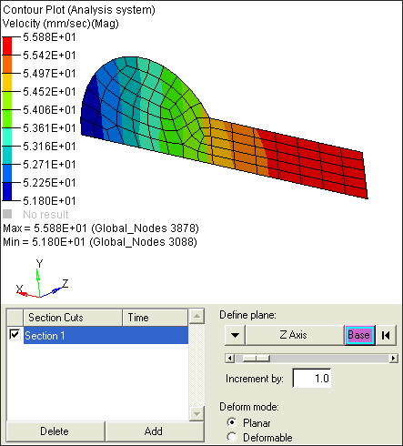
Section cut of velocity results at the exit
|
| 1. | After the nominal run is complete, in HyperStudy, click on Next to continue to create Responses. |
| 2. | Click on Add Response and accept the default for Label and Variable. |
| 3. | Click on Expression to display the Expression Builder. |
| 4. | Click on Add to specify Vector_1 and V_1. |
| 5. | Click the Open File icon under the Vector resource file field and select HX_0452.rsp. |
| 6. | In the Request: field, select Exit_1. |
| 7. | In the Component: field, select Velocity. |
| 8. | Click on Copy and Paste to add Vector_2 and V_2. |
| 9. | In the Request: field, select Exit_2. |
| 10. | In the Component: field, select Velocity. |
| 11. | Select Vector_2 and V_2 and click on Apply. This adds the vector to the response expression. |
| 13. | Select Vector_1 and V_1 and click on Apply. This completes the response expression. |
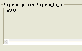
| 14. | Click Evaluate expression. |
| 15. | Notice a value of 1.04043 is displayed. This indicates for a nominal run, v_2/v_1 = 1.04043 |
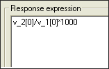
| 16. | Multiply the expression by 1000 to make it larger. |
| 19. | Click Continue to... and select Optimization Study. |
| 20. | Click on Add Optimization.... |
| 21. | Accept the default values. |
| 22. | In the Optimization Engine: field, select Adaptive Response Surface Method. |
| 23. | Click on Next three times to go to Objectives under Optimization Study. |
| 24. | Click Add Objective... and accept the default. |
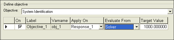
| 25. | Change the Objective: field to System Identification. |
| 26. | Specify the Target Value as 1000. HyperStudy uses this and optimizes the solution in such a way that the flow at Exit_1 is as close to flow at Exit_2 by adjusting the bearing length for each iteration. |
| 27. | Click Launch Optimization. |
| 28. | Click Yes to the message, "Do you wish to skip the solver run for starting point and extract results from nom_run?" |
|
| 1. | Go to the post-processing tab under Optimization Study. |
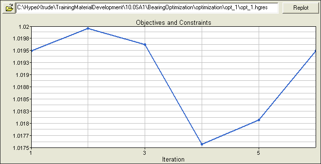
| 2. | Select the Optimization History Plot tab in the center. |
| 3. | Select Resp. The plot shows the Objective function changing for each iteration. You can see that the Objective function starts with 1040 from the nominal run and the optimization stops when the target value reaches 1002. This indicates that the optimization was successful and it could come up with optimal values for bearing length, which gives a velocity closer to uniform at the exit. |
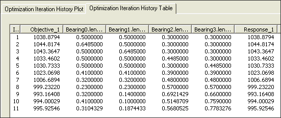
| 4. | Click on the Optimization History table to the right of optimization history plot. This shows the objective function and the bearing lengths used for each iteration. The table indicates that for iteration 11 the flow at Exit_1 and Exit_2 is the same. This means that the velocity of the profile as it exits the die is uniform, which was the goal of the exercise. Iteration 11 has the data files and the results for the optimum bearing lengths. |
| 5. | Load the HX_0452.h3d file from Iteration 11 (from the \optimization\opt_1\run11 directory) into HyperView. |
| 6. | Turn off the display of all components other than the Profile3D component in HyperView. |
| 7. | Create a section cut similar to Step 4. |
|
Notice that the velocity from the optimization run is more uniform. Also, the objective function used for the optimization dictates how accurate the results are from the optimization. For this, optimization averages velocities in the rectangular and semi-circular section and uses them in the objective function.
|
Return to Metal Extrusion Tutorials


