HX-1351: Shape Optimization

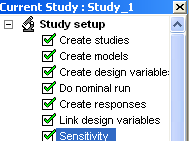
In this tutorial, you will learn how to:

•	Load a HyperMesh file and inspect a model

•	Open HyperStudy through a link in HyperXtrude

•	Add design variables into HyperStudy and perform the nominal run

•	Post-process the nominal run results

•	Perform shape optimization using HyperStudy

•	Post-process the results from the optimization

The purpose of this tutorial is to perform a shape optimization using HyperXtrude and HyperStudy and to ensure that the difference of velocity at the exit is reduced or, ideally, uniform. Shape variables are used as design variables for the optimization with the objective to balance the flow at the exit.

HyperXtrude > has a direct link with HyperStudy that allows the design variables from HyperXtrude to be transferred to HyperStudy to perform the shape optimization. To perform a shape optimization, a HyperXtrude model having results which need to be optimized is required. The model needs to have the shape variables defined. HyperStudy is launched from HyperXtrude, and during the optimization, there is constant communication between HyperXtrude, the solver and HyperStudy.

HX_1351_01

The model files for this tutorial are located in the file mfs-1.zip in the subdirectory \hx\MetalExtrusion\HX_1351. See Accessing Model Files.

To work on this tutorial, it is recommended that you copy this folder to your local hard drive where you store your HyperXtrude data, for example, “C:\Users\HyperXtrude\” on a Windows machine. This will enable you to edit and modify these files without affecting the original data. In addition, it is best to keep the data on a local disk attached to the machine to improve the I/O performance of the software.

•	Tutorial file: HX_1351.hm

1.	Select Start Menu > All Programs > Altair HyperWorks > Manufacturing Solutions > HyperXtrude to launch the HyperXtrude user interface. The User Profiles dialog appears with Manufacturing Solutions as the default application.

2.	Select HyperXtrude and Polymer_Processing from the pull-down menu.

Click OK.

4.	On the File menu, click Open.

5.	Browse to the file HX_1351.hm.

6.	Click Open.

7.	Click the Shaded Elements and Mesh Lines icon .

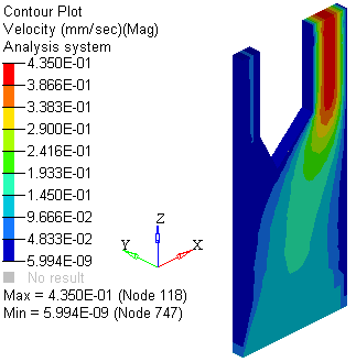
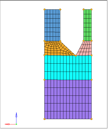
This is a simple two out model for shape optimization. The velocity across small and large sections needs to be uniform.

HX_1351_00

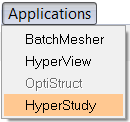
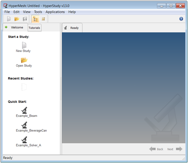
1.	On the Applications menu, click HyperStudy.

HX_1351_02

2.	HyperStudy opens with the interface shown below:

HX_1351_02a

1.	Click on File > New, or click New in the toolbar. The HyperStudy - Add dialog appears.

HX_1351_03

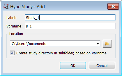
2.	Accept Study_1 for Label, and s_1 for Variable.

3.	Browse to the location of the directory where the HyperMesh file is located. This location is where the files for the nominal run and the optimization will be written.

4.	Click OK. A new study is created and the HyperStudy - Add Study dialog closes.

HX_1351_05

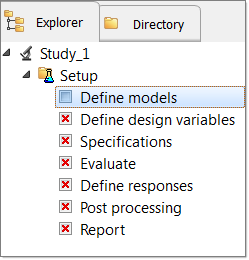
5.	Click Next twice to continue to the Define models step, or click Define models in the study Explorer.

HX_1351_05a

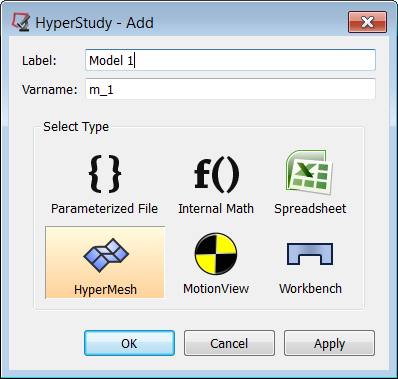
6.	Click Add Model. The HyperStudy - Add dialog appears.

7.	Provide a Label: and a variable name (Varname:), and then select HyperMesh as the model type.

8.	Click OK to add a new HyperMesh model to the Define models table, and to close the HyperStudy - Add dialog.

HX_1351_06

9.	Click Import Variables to import the design variables from the model. The Model Parameters dialog appears. The dialog contains shape variables in HyperXtrude is displayed. These design variables can be added to HyperStudy after specifying the upper and lower bounds for the optimization.

10.	Specify 0.0 as the lower bound.

11.	Specify 1.0 as the upper bound.

12.	Activate both Apply to all selected items checkboxes.

13.	Expand Shape under HyperMesh Model Parameters and select all the shape variables.

14.	Click Add to add the shape variables as HyperStudy parameters.

HX_1351_07

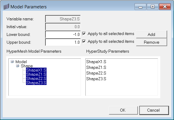
15.	Click OK. The shape variables from HyperXtrude are added as design variables into HyperStudy.

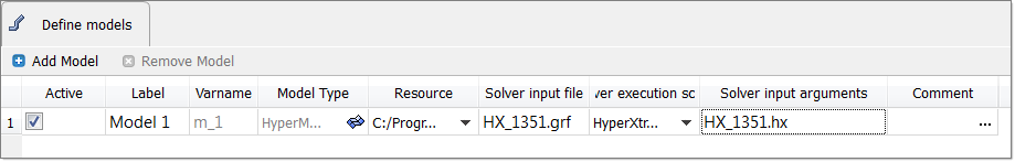
16.	In the Solver input file column for Model_1, enter HX_1351.grf.

17.	Click on Solver execution script > HyperXtude (hx).

18.	In the Solver input arguments field, enter HX_1351.hx.

HX_1351_09

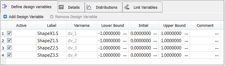
19.	Click Next to continue on to the Define design variables step.

HX_1351_09a

20.	Click Next to continue on to the Specifications step.

21.	In the Specifications table, make sure the Mode is set to Nominal Run and then click Apply.

22.	Click Next to continue on to the Evaluate step.

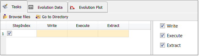
23.	Make sure the task manager settings Write, Execute, and Extract are all checked. This will create a folder with a name nom_run and a subfolder m_1 inside it under the specified directory (selected above). It also writes the input files for the solver inside m_1.

HX_1351_09b

24.	Click Evaluate Tasks.

25.	Click Next to continue on to the Define responses step, where you will export the HyperXtude data files and run the analysis in batch mode.

1.	Load the HX_1351_000.h3d model into HyperView.

1.	After the nominal run is complete, click Next to go to Create responses.

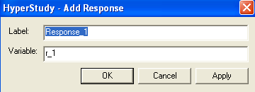
2.	Click Add Response and accept the defaults for Label and Variable.

HX_1351_11

3.	Click Expr Builder....

4.	Click Add to specify Vector_1 and V_1.

5.	Under vector resource file, browse to HX_1351.rsp.

6.	In the Request: field, select out_small.

7.	In the Component: field, select Velocity.

8.	Click copy and paste to add Vector_2 and V_2.

9.	In the Request: field, select out_large.

10.	In the Component: field, select Velocity.

HX_1351_12

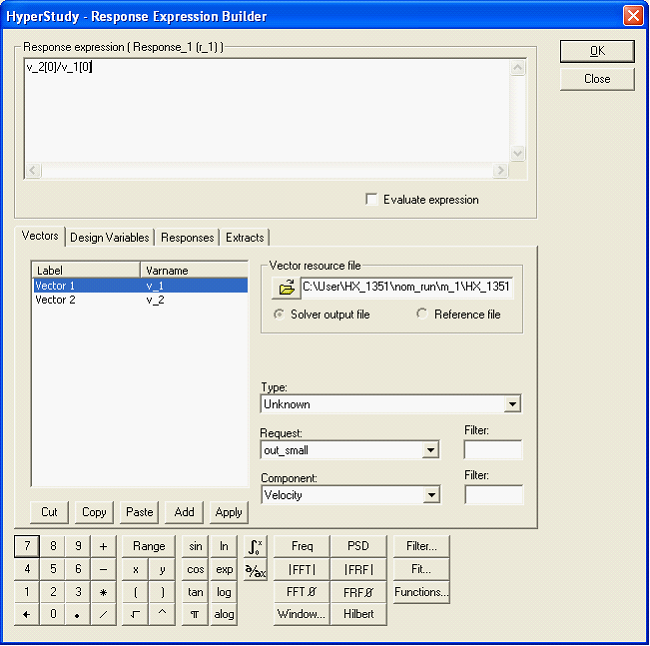
11.	Select Vector_2 and V_2 and click Apply. This adds the vector to the response expression.

12.	Click on "/"

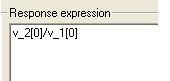
13.	Select Vector_1 and V_1 and click Apply. This completes the response expression. Notice the equation created in the Response expression window.

HX_1351_13

14.	Click OK to close the Response expression window and click Next twice.

HX_1351_14

15.	Click Continue To and select Optimization Study.

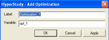
16.	Click Add Optimization....

17.	Accept the default values and click OK.

HX_1351_15

18.	In the Optimization Study: field, select Adaptive Surface Response Method.

19.	Click Next twice to go to Objectives under Optimization Study.

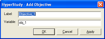
20.	Click Add Objective... and accept the default.

HX_1351_16

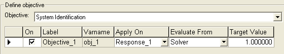
21.	Change the Objective: field to System Identification.

22.	Specify the Target Value as 1.000. HyperStudy uses this and optimizes the solution such a way that the flow at out_small is as close to flow at out_large by adjusting the shape variable values for each iteration.

HX_1351_17

23.	Click Launch Optimization.

24.	Click Yes to the message, "Do you wish to skip the solver run for starting point and extract results from nom_run?"

1.	Under Optimization study, click Post processing.

HX_1351_18

2.	Select the Optimization History Plot tab in the center.

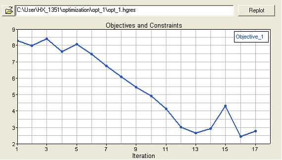
Select Resp. The plot shows the Objective function changing for each iteration. You can see that the Objective function starts with 8.2829 from the nominal run and the optimization stops when the target value is close to 3. This indicates that the optimization was successful and it could come up with better values for shape variables which gives less difference of velocities at the exit.

4.	Click the Optimization History table to the right of optimization history plot. This shows the objective function and the shape variable values used for each iteration. The table indicates that for iteration 18 the difference of flow at out_small and out_large is reduced.

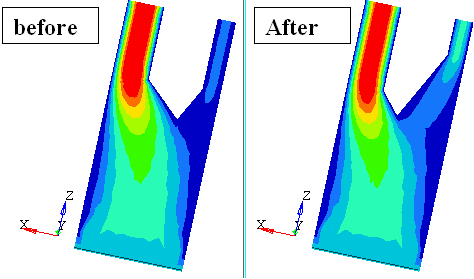
5.	Load the HX_1351_000.h3d file from Iteration18 into HyperView. Notice the shape difference before and after optimization.

HX_1351_19

6.	To achieve ideal uniform velocities at both exits, different shape variables will need to be created in the optimization setup. Refer to HyperMorph tutorials for creating a variety type of shape variables.

Notice that the velocity from the optimization run is more uniform. Also another thing to note is the objective function used for the optimization dictates how accurate the results are from the optimization. For this optimization average velocities in the out_small and out_large section were used in the objective function.

Return to Polymer Processing Tutorials