Example: Optimization Using Radioss
In this example, you will learn how to perform an optimization using the Design Explorer workflow.
The model used for the optimization is a B-Pillar cut from a full car model. An initial velocity is applied to a rigid cylinder in the transverse (Y) direction.
The objective of the optimization is to minimize the mass of the B-Pillar while constraining the maximum displacement of a node on the inner panel to less than 19.7 mm.
- BPillar.hm
Open the Model
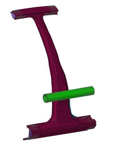
Figure 1.
Create an Exploration
-
From the Design Explorer ribbon, Exploration tool group, click the
Create Explorations tool.

Figure 2.The Explorations dialog opens. -
Click
 then select Optimization.
-
In the Study Path field, browse to and select the folder to store your
optimization.
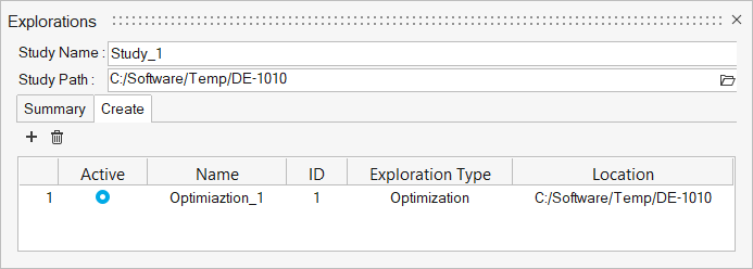
Figure 3. -
From the Exploration tool group, click the Design
Explorer tool.

Figure 4.The Design Explorer browser opens. You can see the newly created optimization exploration. Additional exploration entities will appear here as well.
Create the Exploration Inputs
-
From the Design Explorer ribbon, click the Gauge
tool.

Figure 5. -
In the modeling window, select the green
Inner property.
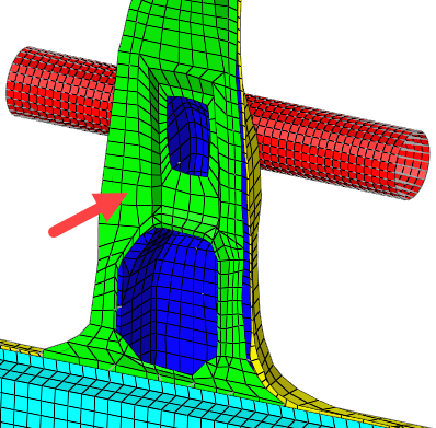
Figure 6. -
In the microdialog, click the drop-down on the left and
select Bounds=, then set the upper bound to
0.5 and the lower bound to
3.0.
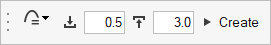
Figure 7. -
Click Create.
A gauge design variable is created.
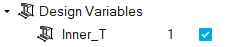
Figure 8. -
On the guide bar, click
 .
The Advanced Selection dialog opens.
.
The Advanced Selection dialog opens. -
In the microdialog, click
Create.
A second gauge design variable is created.
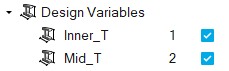
Figure 9. -
On the ribbon, hover over the Gauge tool then click the satellite icon
 .
The Review Inputs dialog opens.
.
The Review Inputs dialog opens. -
For the Mid_T design variable, modify the Lower Bound and Upper Bound to
0.5 and 3.0
respectively.
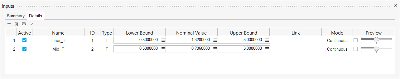
Figure 10.
Create the Exploration Responses
-
From the Design Explorer ribbon, click the Mass/Volume
tool.

Figure 11. -
On the guide bar, click
 .
A mass response is created.
.
A mass response is created. -
Click the Disps. tool.

Figure 12. -
On the guide bar, click .
-
In the microdialog, expand the options and select
Y from the Response Component drop-down menu.
The displacement response is updated.The optimization now consists of two design variables and two responses.
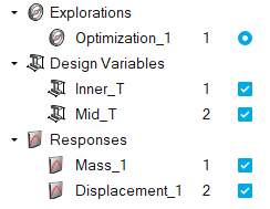
Figure 13.
Create the Objective and Constraint
-
From the Design Explorer ribbon, click the Objectives
tool.

Figure 14. -
On the guide bar, click .
The Advanced Selection dialog opens.
-
Click the Constraints tool.

Figure 15. -
On the guide bar, click .
The Advanced Selection dialog opens.
Evaluate the Exploration
-
From the Design Exploration ribbon, Evaluate tool group, click the
Evaluate tool.

Figure 16.The Evaluate dialog opens. -
Click Export then click
Run.
The optimization is evaluated. In this case, there will be a nominal run plus 20 optimization runs.
This may take a few minutes depending on your computer.
When the evaluation is complete, the Evaluation Status dialog should look like the following.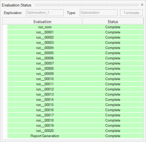
Figure 17.
Review the Evaluation
-
From the Design Exploration ribbon, Evaluate tool group, click the
Results Explorer tool.

Figure 18.The Results Explorer opens. -
Review the Summary table, which shows the input, objective, and constraint
values for each run of the optimization.
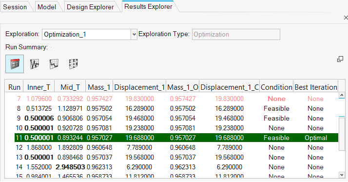
Figure 19.The values for the optimal thicknesses found from the optimization are indicated by a green background, and additional feasible designs are indicated as well. Orange font indicates that at least one constraint is nearly violated. Red font indicates runs with at least one violated constraint.
-
In the Results Explorer, click the Iteration Plot button
(
 ).
).
-
In the Entity selection area, check the Mass_1 response.
Notice how the objective varied and was minimized during the optimization.
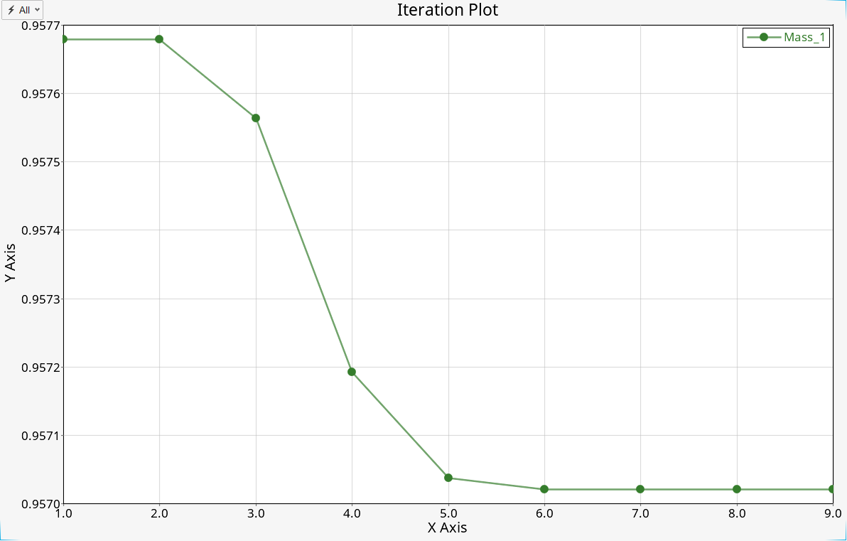
Figure 20.