Example: DOE Using OptiStruct
In this example, you will learn how to perform a design of experiments (DOE) using the Design Explorer workflow.
Before you begin, copy the model used in this example from <HyperWorks
Installation Directory>/tutorials/hwdesktop/hwx/ to your working directory.
- bikeFrame.hm
Open the Model
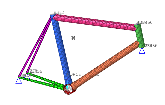
Figure 1.
Create an Exploration
-
From the Design Explorer ribbon, Exploration tool group, click the
Create Explorations tool.

Figure 2.The Explorations dialog opens. -
Click
 then select DOE.
-
In the Study Path field, browse to and select the folder to store your
DOE.
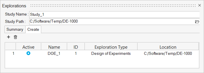
Figure 3. -
From the Exploration tool group, click the Design
Explorer tool.

Figure 4.The Design Explorer browser opens. You can see the newly created optimization exploration. Additional exploration entities will appear here as well.
Create the Exploration Inputs
-
From the Design Explorer ribbon, click the Gauge
tool.

Figure 5. -
In the microdialog, click
Create.
Two gauge design variables are created.
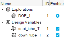
Figure 6.
Create the Exploration Responses
-
From the Design Explorer ribbon, click the Mass/Volume
tool.

Figure 7. -
On the guide bar, click
 .
A mass response is created.
.
A mass response is created. -
Click the Disps. tool.

Figure 8. -
In the modeling window, select the node where the crank
load is applied.
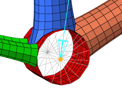
Figure 9. -
In the microdialog, click
 .
An Entity Editor window appears.
.
An Entity Editor window appears.- Change the response name to Crank.
- From the Response Component drop-down menu, select Z.
- Click Close.
The displacement response is updated. -
On the guide bar, click .
-
Select the node where the seat sits.
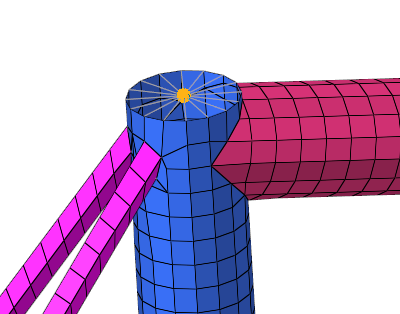
Figure 10.A second displacement response is created. -
In the microdialog, click .
An Entity Editor window appears.
- Change the response name to Seat.
- From the drop-down menu, select MAG.
- Click Close.
The displacement response is updated. -
On the guide bar, click
 .
.
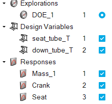
Figure 11.
Evaluate the Exploration
-
From the Design Exploration ribbon, Evaluate tool group, click the
Evaluate tool.

Figure 12.The Evaluate dialog opens. -
Click Export then click
Run.
The DOE is evaluated. In this case, there will be a nominal run plus four DOE runs.
This may take a few minutes depending on your computer.
When the evaluation is complete, the Evaluation Status dialog should look like Figure 13.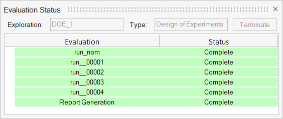
Figure 13.
Review the Evaluation
-
From the Design Explorer ribbon, Evaluate tool group, click the
Results Explorer tool.

Figure 14.The Results Explorer browser opens. -
Review the Summary table, which shows the input and response values for each
run of the DOE.
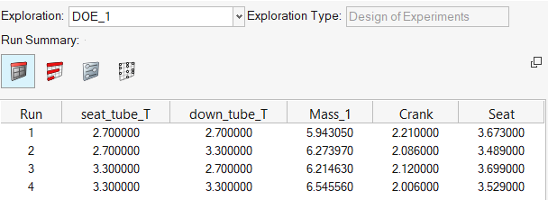
Figure 15. -
Right-click on any row in the Summary table and select Load
Results.
A HyperView window opens, and the results contour from the selected run is displayed.
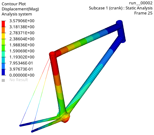
Figure 16. -
In the Results Explorer, click the Linear Effects button
(
 ).
).
-
From the Select response drop-down menu, select
Crank.
The Linear Effects plot shows the relative contribution of each design variable on the crank displacement response.
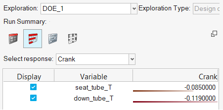
Figure 17.Note: Notice the negative correlation between the gauge design variables and the displacement response. This indicates that an increase in the gauge of the component will result in a corresponding decrease to the displacement response. In addition, the relative effect of a change to the down tube thickness will be greater than a similar change to the seat tube thickness.In addition, the effects contour is mapped onto the model itself in the graphics area for visualization.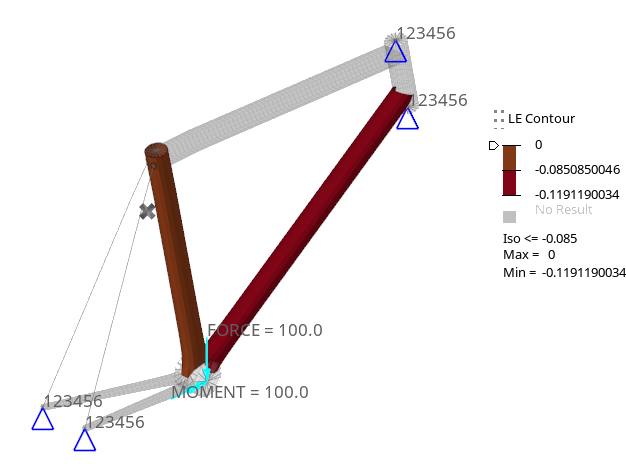
Figure 18.Note: This can be quite useful when dealing with a larger number of design variables.In the table as well as on the model, positive effects – indicating a positive relationship between the design variable and response – are shown in shades of blue, whereas negative effects – indicating an inverse relationship between the design variable and response – are shown in shades of brown.
-
As an exercise, try creating a similar DOE where the gauge of every component
is a design variable. Your DOE and reports should look something like the
following (your actual values will vary, based on your specific design variable
bounds choices).
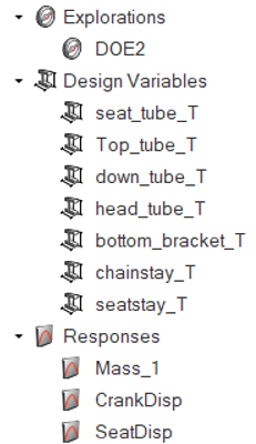
Figure 19.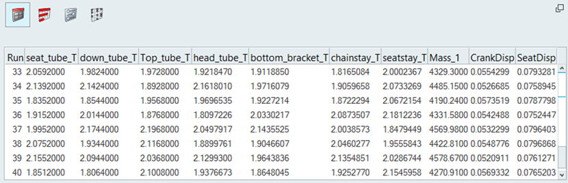
Figure 20.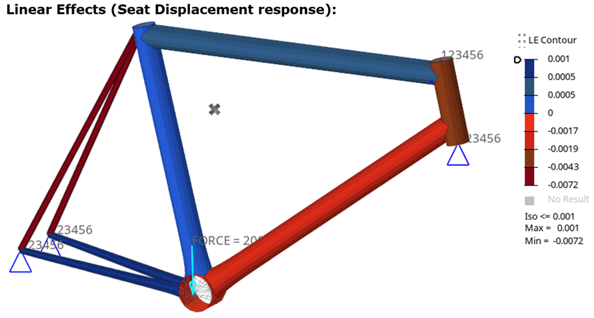
Figure 21.