HS-5020: Stochastic Study of a Cantilever I-beam
In this tutorial, you will complete a simple Stochastic study to investigate uncertain parameters of a cantilever I-beam model defined with four variables and four functions.
Before you begin, copy HS-5020.hstx
from <hst.zip>/HS-5020/ to your working directory.
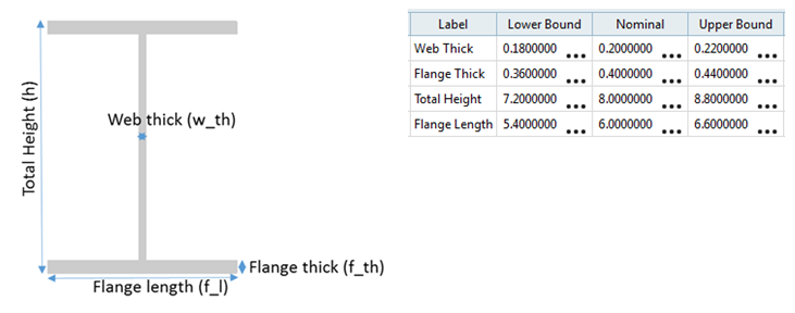
Figure 1.
Run a Stochastic Study
In this step, you will run a Stochastic study and review the evaluation scatter.
In this study, you will consider w_th, f_l and f_th as Random parameters (uncertain, not controllable by design) and h as Design with Random parameter (uncertain but controllable by design).
-
Modify input variables.
-
In the Distribution Role column, select Design with
Random for Total Height.
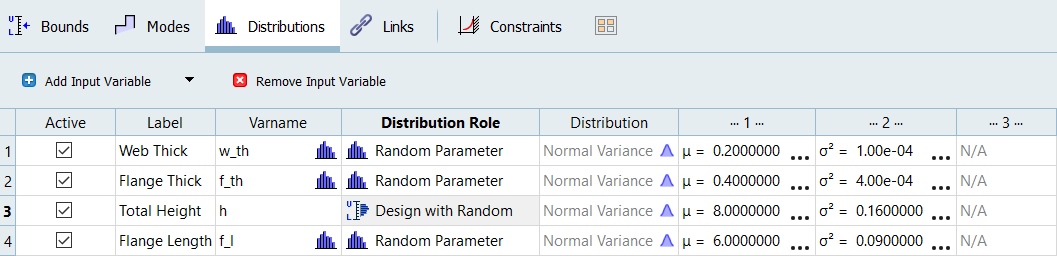
Figure 2. -
In the Distribution column, verify Normal
Variance is selected for all active variables.
The Distribution column allows you to select the Distribution type. Normal Variance (shown in Figure 3) means parameters could take random values following normal distribution around their nominal values (µ).
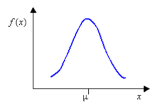
Figure 3.
-
In the Distribution Role column, select Design with
Random for Total Height.
-
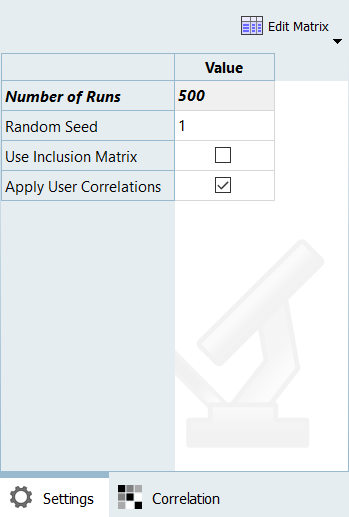
In the Settings tab, change the Number of Runs to
500.
-
Review the scatter plots for Total Height and Web Thick.
The Evaluation scatter shown in Figure 4 presents the sampling for Total Height and Web Thick. Due to the Design with Random distribution role the sampling for Total Height is truncated to only samples which fall between the upper and lower bounds.
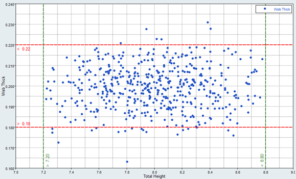
Figure 4.
Review Post-Processing Results
In this step, you will review the evaluation results within the Post-Processing step.
-
Review the histograms of the stochastic results.
Figure 5 shows the histograms of Total Height and Web Thick values distributions. Each blue bin represents the frequency of runs yielding a sub-range of response values. Notice the Total Height histogram has no tails at the extremities because of the truncated sampling. The probability densities (red curves) indicate the relative likelihoods of the variables to take particular values. A higher value indicates that the values are more likely to occur. The cumulative distributions (green curves) indicate what percentage of the data falls below the value threshold.
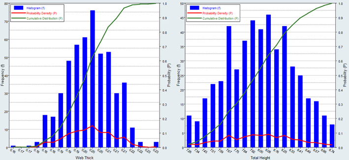 Figure 5.
 -
Identify the eventual outliers.
Note: There are no outliers for Total Height because of the truncated sampling.
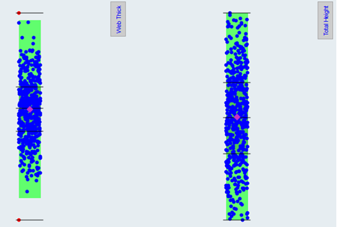
Figure 6. -
Create another reliability by repeating step 8 with the following
changes:
- Set Response to Disp (r_4).
- Set Bound Type to <=.
- For Bound Value, enter 4.41e-05.
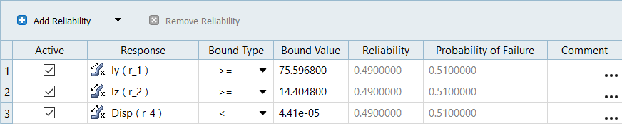
Figure 7. -
Review the graphs.
Figure 8 show the reliabilities for the values Web Thick and Total Height could take.
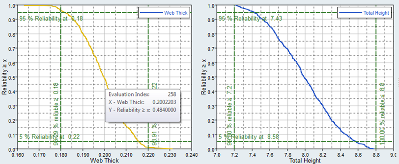
Figure 8.