Learn how to create a Lookup model to link to tabulated data in an external
.csv file, run a DOE of type Run Matrix to import the data in the
lookup .csv file, and build a predictive model using FAST (Fit
Automatically Selected by Training).
Before you begin, copy the model files used in
this tutorial from <hst.zip>/HS-3015/ to your working
directory.
Review CSV Data
Open the FAST_data.csv file and review its contents.
The .csv file contains two variables (x and y) and
three responses.
Perform the Study Setup
Start HyperStudy.
Start a new study in the following ways:
From the menu bar, click File > New.
On the ribbon, click .
In the Add Study dialog, enter a study name, select a
location for the study, and click OK.
Go to the Define Models step.
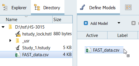
Add a Lookup model by dragging-and-dropping the
FAST_data.csv file from the Directory into the work
area.
Figure 1.
Import variables.
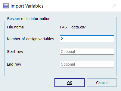
Click Import Variables.
The Import Variables dialog
opens.
In the Number of design variables field, enter
2.
Click OK.
The input variables are expected in the first two columns, and the remaining
columns are interpreted as output responses. Figure 2.
Go to the Define Input Variables step.
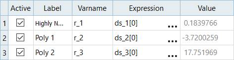
Review the input variables.
The bounds of the input variables are based on the
FAST_data.csv file’s contents. The nominal values
are set to the first entry in the .csv file. Figure 3.
Perform Nominal Run
Go to the Test Models step.
Click Run Definition.
An approaches/setup_1-def/ directory is created
inside the study Directory. The
approaches/setup_1-def/run__00001/m_1 directory
contains the input file, which is the result of the nominal run.
Review Output Responses
Go to the Define Output Responses step.
Review the output responses.
One output response is named Highly Nonlinear and two are
polynomials. Figure 4.
Run a Run Matrix DOE
Add a DOE.
In the Explorer, right-click and select
Add from the context menu.
In the Add dialog, select
DOE and click OK.
Go to the DOE 1 > Specifications step.
In the work area, set the Mode to Run Matrix.
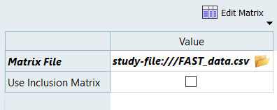
From the Settings tab, Matrix File field, navigate to your working directory
and select the FAST_data.csv file.
Figure 5.
Click Apply.
The DOE matrix populates with the input variable values from the
FAST_data.csv file.
Go to the DOE 1 > Evaluate step.
Click Evaluate Tasks.
Run FAST Fit
Add a Fit.
In the Explorer, right-click and select
Add from the context menu.
In the Add dialog, select
Fit and click OK.
Import matrix.
Go to the Fit 1 > Specifications step.
Click Add Matrix.
In the work area, set Matrix Source to Doe 1
(doe_1).
Click Apply.
Define specifications.
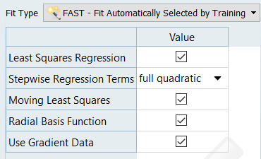
Verify that the Fit Type assigned to each output response is FAST – Fit
Automatically Selected by Training.
Figure 6.
By default, FAST automatically selects the best Fit type from all
available Fits. You can manually select the Fit types FAST can choose by
highlighting one or more responses in the work area and selecting Fits
from the Settings tab. Figure 7.
Click Apply.
Evaluate tasks.
Go to the Fit 1 > Evaluate step.
Click Evaluate Tasks.
Note: The choices for the best available Fit vary for each output
response, which can cause these loops to be time consuming compared
to when you select a single specific Fit. The steps for each output
response are mutually exclusive, therefore you can use the
Multi-Execution option to accelerate this process.
Go to the Fit 1 > Post-Processing step.
Review diagnostics.
Click the Diagnostics tab.
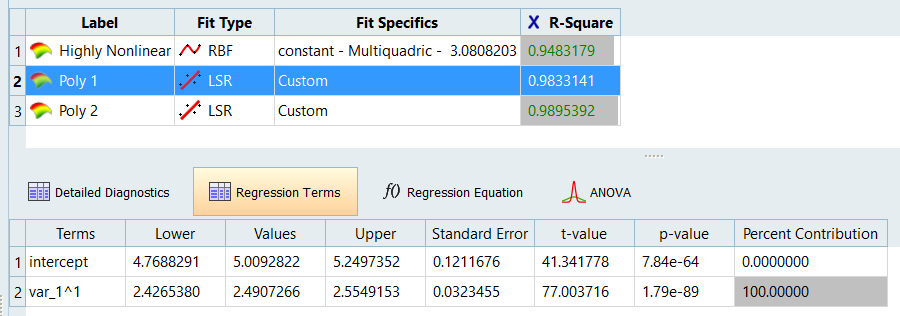
The Highly Nonlinear response uses RBF, while the other
responses use LSR. In each case, FAST selected the specifics to have the
highest validation R-square value. The R-Square can be interpreted as
the % of the data’s variance that can be explained by the model. Figure 8.
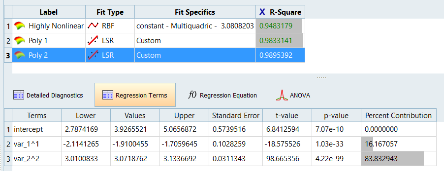
Click Regression Terms and compare Poly1 and
Poly2 by selecting them individually in the work area.
Poly1 and Poly2 are using stepwise regression, which means that
the coefficients of the regression are reduced to a minimal set that
sufficiently models the data. Poly1 uses only x, whereas Poly2 uses x
and y^2. Figure 9. Poly1 Figure 10. Poly2
If required, copy the data from the Fit Type and
Fit Specifics columns in the Diagnostics
table and paste it into the Fit Type and
Fit Specifics columns in the Specification
step.
This step explicitly sets the Fit specifications to the results
determined from FAST; if the Fit must be re-run, this step can save time
because FAST does not need to search for the best settings.
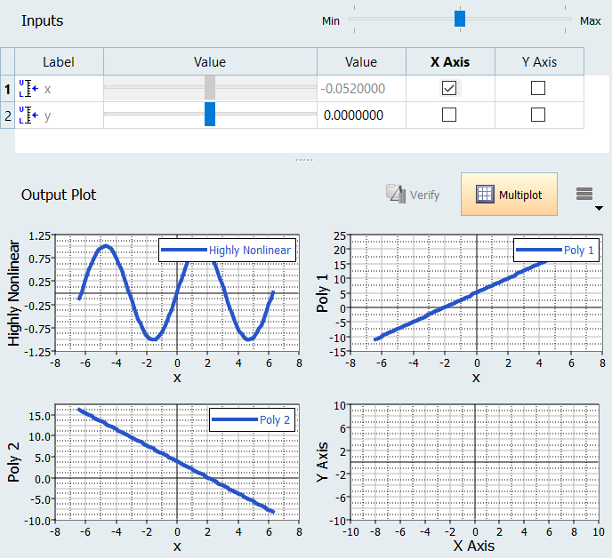
Click the Trade-Off Tab to plot all the functions and
see the predicted versus the known data points.
In each case, the Fit model follows the data closely regardless of the
sinusoidal functions in the Highly Nonlinear response to the simple planar data
of the polynomial responses. Figure 11.
 .
.