ACU-T: 3201 Solar Radiation and Thermal Shell Tutorial
Prerequisites
This tutorial introduces you to setting up a CFD simulation involving solar radiation and thermal shells using AcuSolve and HyperMesh. Prior to starting this tutorial, you should have already run through the introductory tutorial, ACU-T: 1000 HyperWorks UI Introduction, and have a basic understanding of HyperMesh, AcuSolve, and HyperView. To run this simulation, you will need access to a licensed version of HyperMesh and AcuSolve.
Prior to running through this tutorial, copy HyperMesh_tutorial_inputs.zip from <Altair_installation_directory>\hwcfdsolvers\acusolve\win64\model_files\tutorials\AcuSolve to a local directory. Extract ACU-T3201_SolarRadiation.hm and SolarLoad.dat from HyperMesh_tutorial_inputs.zip.
Since the HyperMesh database (.hm file) contains meshed geometry, this tutorial does not include steps related to geometry import and mesh generation.
Problem Description

Figure 1.
Solar Radiation Parameters
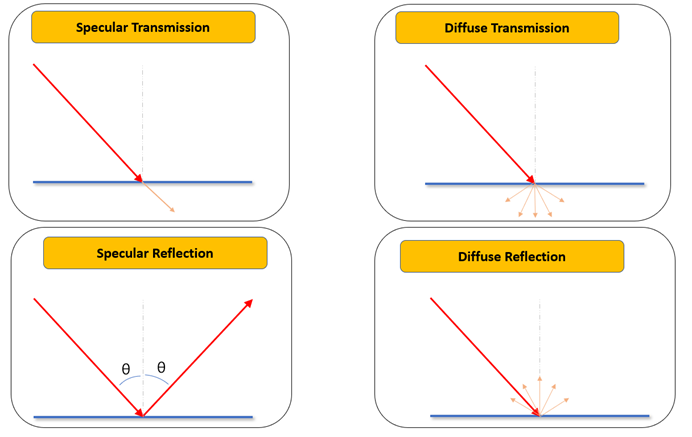
Figure 2.
- Specular transmissivity
- Diffuse transmissivity
- Specular reflectivity
- Diffuse reflectivity
- Absorptivity
- Angle of incidence
For the solar radiative heat fluxes to be computed, a solar radiation surface needs to be defined on that given surface.
In this tutorial, the solar flux loading is given in the form of a data file which was generated using the acuSflux script available in AcuSolve. The script can be used to generate a data file with a four-column array of solar flux vector data values. The piecewise linear type is used in this tutorial to emulate the pattern of sunrise to sunset over the atrium.
For example, to generate the solar load data file for a location with known geological coordinates, enter the following command in the AcuSolve Command Prompt: acuSflux -time "dec-3-2019 11:00:00" -tinc 1800 -nts 25 -lat 42.6064 -lon -83.1498 -ndir "1,0,0" -udir "0,0,1"
- time
- The start time in GMT (ex: “dec-3-2019 21:00:00”)
- tinc
- The time increment in seconds
- nts
- Number of discrete time steps
- lat
- Latitude coordinates of the location in degrees North (ex: 45.112 or -37.56 (equal to 37.56 S))
- lon
- Longitude coordinates of the location in degrees East (ex: 86.26 or -54.84 (equal to 54.84 W))
- ndir
- The north direction unit vector in model coordinates (should be enclosed in double quotes) (ex: “0,1,0”)
- udir
- The upward direction unit vector in model coordinates (should be enclosed in double quotes) (ex: “0,1,0”)
Thermal Shell Modeling
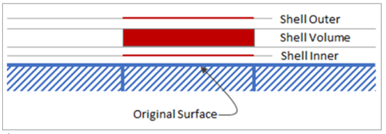
Figure 3.
When defining a thermal shell on a surface, two sets of boundary conditions are needed. One for the Primary Wall surface i.e. Shell Inner and one for the Shell Outer Wall surface. In this tutorial, a solar radiation surface will be defined on the outer shell surface so that it receives solar heat flux, whereas the inner shell surface will be modeled as a default wall.
Open the HyperMesh Model Database
-
Click the Open Model icon
 located on the standard toolbar.
The Open Model dialog opens.
located on the standard toolbar.
The Open Model dialog opens.
Set Up the Simulation Parameters
Set the General Simulation Parameters
-
Set the Turbulence model to Laminar (if not set
already).
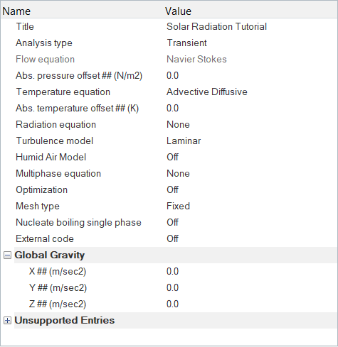
Figure 4.
Specify the Solver Settings
-
Verify that the Flow and Temperature fields are turned
On.
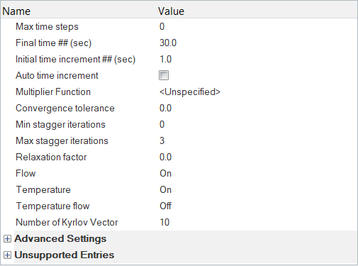
Figure 5.
Set the Solar Radiation Parameters
-
Leave the remaining options as default.
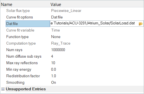
Figure 6.
Assign Material Properties and Boundary Conditions
Create the Solar Radiation Model
-
Set the Diffusive reflectivity to 0.01.
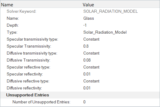
Figure 7.
Assign Material Properties and Boundary Conditions
-
Click Fluid. In the Entity Editor,
- Change the Type to FLUID.
- Set the Material to Air_HM.
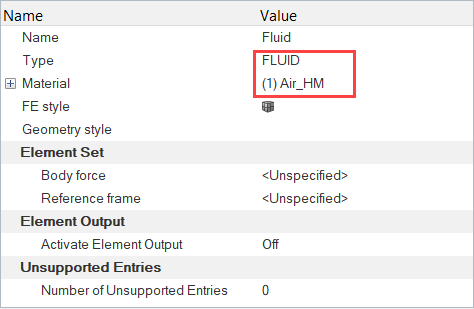
Figure 8. -
Click Walls. In the Entity Editor,
-
Set the Convective heat flux reference temperature to
283.15 K.
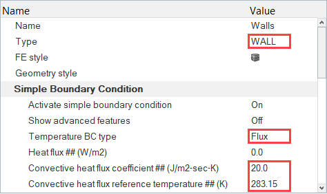
Figure 9. -
Under the Solar Radiation Surface tab, turn on the
Display field. Turn On
the Activate solar radiation surface option. Set the Type to
Outward. Set the Solar radiation model to
Solar Radiation Black Body.
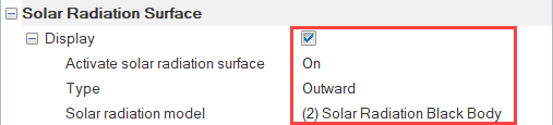
Figure 10. -
Under the Surface Output tab, turn On Surface
Output and set the Nodal time step frequency to
1.
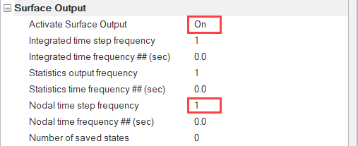
Figure 11.
-
Set the Convective heat flux reference temperature to
283.15 K.
-
Click Inlet. In the Entity Editor,
-
Set the Temperature of the incoming fluid to
295.35 K.
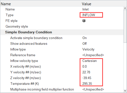
Figure 12. -
Under the Solar Radiation Surface tab, turn on the
Display field. Turn On
the Activate solar radiation surface option. Set the Type to
Outward. Set the Solar radiation model to
Solar Radiation Black Body.
Figure 13.
-
Set the Temperature of the incoming fluid to
295.35 K.
-
Click Outlet. In the Entity Editor, change the Type to OUTFLOW.
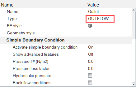
Figure 14. -
Click Glass. In the Entity Editor,
-
Set the Convective heat flux reference temperature to
283.15 K.
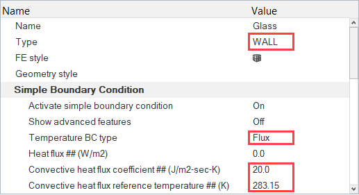
Figure 15. -
Under the Solar Radiation Surface tab, turn on the
Display field. Turn On
the Activate solar radiation surface option. Set the Type to
Both. Set the Solar radiation model to
Glass.
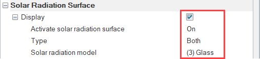
Figure 16. -
Under the Surface Output tab, turn On Surface
Output and set the Nodal time step frequency to
1.
Figure 17.
-
Set the Convective heat flux reference temperature to
283.15 K.
-
Click Floor. In the Entity Editor,
- Verify that the Type is set to WALL and the Temperature BC type is set to Flux.
- Under the Solar Radiation Surface tab, turn on the Display field. Turn On the Activate solar radiation surface option. Set the Type to Inward. Set the Solar radiation model to Solar Radiation Black Body.
- Under the Surface Output tab, turn On Surface Output and set the Nodal time step frequency to 1.
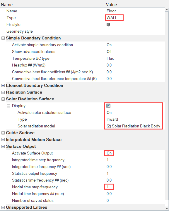
Figure 18. -
Click Glass_walls. In the Entity Editor,
-
For the Primary Wall boundary condition, leave the default values
unchanged.
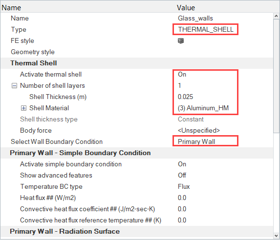
Figure 19.
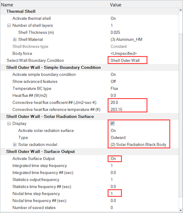
Figure 20. -
For the Primary Wall boundary condition, leave the default values
unchanged.
-
Click Chair. In the Entity Editor,
- Verify that the Type is set to WALL.
- Under the Solar Radiation Surface tab, turn on the Display field. Turn On the Activate solar radiation surface option. Set the Type to Default. Set the Solar radiation model to Solar Radiation Black Body.
- Under the Surface Output tab, turn On Surface Output and set the Nodal time step frequency to 1.
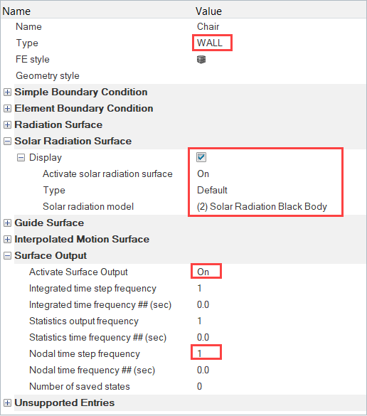
Figure 21.
Set Nodal Initial Conditions
- In the Solver Browser, click 03.NODAL_INITIAL_CONDITION under 01.Global.
- In the Entity Editor, change the Default value of Temperature to 288.15 K.
Define Nodal Output Frequency
- In the Solver Browser, expand 17.Output then click NODAL_OUTPUT.
- In the Entity Editor, set the Time step frequency to 1.
- Activate the Output initial condition checkbox.
- Save the model.
Compute the Solution
-
Click
 on the ACU toolbar.
The Solver job Launcher dialog opens.
on the ACU toolbar.
The Solver job Launcher dialog opens.
Post-Process the Results using HyperView
In this step, you will create an animation of solar heat flux and temperature over run time. Once the solver run is complete, close the AcuProbe and AcuTail windows. In the HyperMesh Desktop window, close the AcuSolve Control tab and save the model.
Switch to the HyperView Interface and Load the AcuSolve Model and Results
-
In the HyperMesh Desktop window, click the
ClientSelector drop-down in the bottom-left corner of
the graphics window.
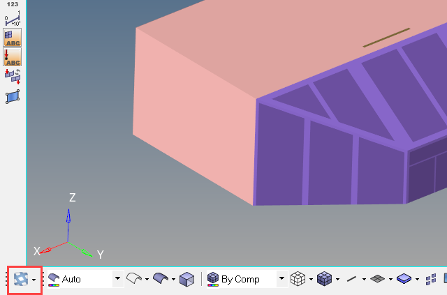
Figure 22. -
In the Load model and results panel, click
 next
to Load model.
next
to Load model.
-
In the Reader Options dialog, set the Reader to
AcuSolve Result Reader and the Extended nodal output
option to Yes then click OK.
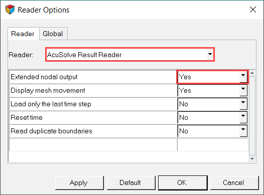
Figure 23.
Create an Animation of Temperature Contour
In this step, you will start by creating an expression for plotting the temperature values in Fahrenheit units. Then, you will create an animation of the magnitude of temperature on the floor, glass_walls and the man surface.
-
Complete the expression by entering the remaining portion of the formula as
shown in the figure below.
Here the term ‘R1.S16’ corresponds to the Temperature (scalar) variable in Kelvin. Variables can be inserted in the expression by selecting the required variable under Table option and then clicking Insert. The actual ID for the scalar variable might be different for your simulation.
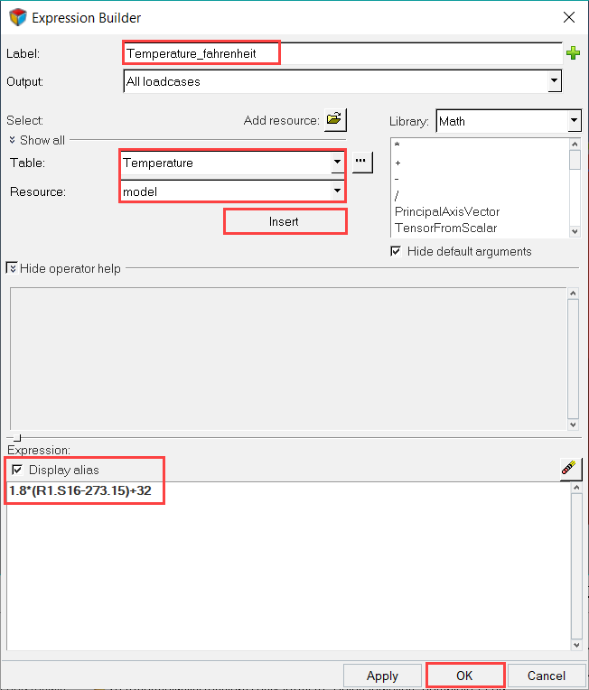
Figure 24. -
In the Results Browser, expand the list of
Components. Turn off the display of all the
components except Floor, Glass_walls Shell
Outer, and Chair surfaces.
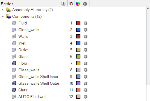
Figure 25. -
Click
 on the Results toolbar to open the Contour panel.
-
In the panel area, under the Display tab, turn off
the Discrete color option.
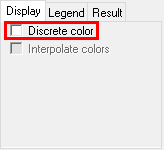
Figure 26. -
Click
 on the Animation toolbar to play the temperature
animation.
on the Animation toolbar to play the temperature
animation.
-
Click the Animation Controls icon
 . In the panel area, set the Max
Frame Rate to 5 Frames/Sec by dragging the slider.
. In the panel area, set the Max
Frame Rate to 5 Frames/Sec by dragging the slider.
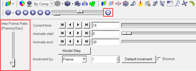
Figure 27.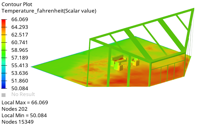
Figure 28.
Create an Animation of Solar Heat Flux
-
Click
on the Results toolbar to open the Contour panel.
-
Click Apply.
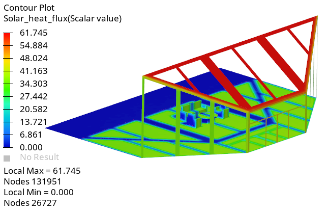
Figure 29. -
On the ImageCapture toolbar, click on the Capture Graphics Area
Video icon
 .
.
Summary
In this tutorial, you learned how to set up and solve a CFD analysis involving solar radiation and thermal shells. You started by importing a HyperMesh model database and set up the simulation parameters and boundary conditions. Once you computed the solution, you post-processed the results using HyperView. Also, you learned how to create expressions in HyperView and build plots using derived results.