ACU-T: 3101 Transient Conjugate Heat Transfer in a Mixing Elbow
Prerequisites
This tutorial provides you instructions for running a transient simulation of a 3D turbulent flow with conjugate heat transfer in a mixing elbow. You should have already run through the ACU-T: 3100 Conjugate Heat Transfer in a Mixing Elbow tutorial and have a basic understanding of HyperMesh, AcuSolve and HyperView. The HyperWorks introductory tutorial, ACU-T: 1000 HyperWorks UI Introduction, gives a basic introduction to HyperWorks and AcuSolve.
Prior to running through this tutorial, copy HyperMesh_tutorial_inputs.zip from <Altair_installation_directory>\hwcfdsolvers\acusolve\win64\model_files\tutorials\AcuSolve to a local directory. Extract ACU-T3101_MixingElbowTransient.hm from HyperMesh_tutorial_inputs.zip.
Since the HyperMesh database (.hm file) contains meshed geometry, this tutorial does not include steps related to geometry import and mesh generation.
Problem Description
This problem is divided into two components, a steady state solution and a transient solution. The schematic of the steady state component is shown below.

Figure 1.
The diameter of the large inlet is 0.1 m, the inlet velocity (v) is 0.4 m/s and the temperature (T) of the fluid entering the large inlet is 295 K. The diameter of the small inlet is .025 m, the velocity is 1.2 m/s, and the temperature of the fluid entering the small inlet is 320 K. The pipe wall has a thickness of 0.005 m. The fluid in this problem is water and the pipe walls are made of stainless steel with a density of 8030 kg/m3, a conductivity of 16.2 W/m-K, and a specific heat of 500 J/kg-K.
The model file for the steady state part of the problem is provided as the input file. Once the steady state solution is computed, it is projected on to the mesh and used as the initial state for the transient simulation. The starting point for the transient portion of the problem is shown schematically in the figure below.
Figure 2.
At 0.2s into the simulation, a cold slug of water is injected at both the inlets and the temperature is ramped down to 283.15 K starting from 0.2 s to 0.4 s. Then it is maintained constant at 283.15 K for 1 sec and then ramped up to initial states from 1.4s to 1.6s. Given a flow path of 0.6356 m, the transit time for the slug is approximately 1.6s. Therefore, our simulation time should be at least 3.2 s to factor in the duration of the slug and transit time. The total simulation time will be 4.5s to allow time for the thermal conditions to return to a steady state.
The temperature change at the large inlet is from 295 K to 283.15 K. At the small inlet, the temperature changes from 320 K to 283.15 K. The ratio of the cold slug temperature to the initial temperature of the large inlet flow is 0.9598. The ratio of the cold slug temperature to the initial temperature of the small inlet flow is 0.8848. These values will be used in creating multiplier functions to model the transient temperatures at the inlets.
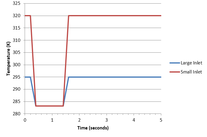
Figure 3.
Open the HyperMesh Model Database
-
Click the Open Model icon
 located on the standard toolbar.
The Open Model dialog opens.
located on the standard toolbar.
The Open Model dialog opens.
Run the Steady State Simulation
In this step, you will run the steady state simulation with the model file provided and then create the nodal initial condition files needed for the transient simulation. Make sure that the visibility of the mesh for all the components is on.
-
Click
 on the ACU toolbar.
The Solver job Launcher dialog opens.
on the ACU toolbar.
The Solver job Launcher dialog opens.
Set the Transient Simulation Parameters
Set the Analysis Parameters
-
Change the Analysis type to Transient in the Entity Editor.
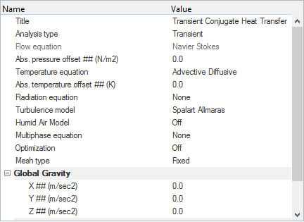
Figure 4.
Specify the Solver Settings
-
Turn Off the Flow and Turbulence fields.
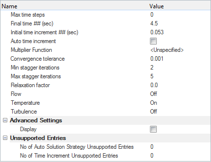
Figure 5.
Set the Nodal Output Frequency
-
Turn On the Output initial condition field.
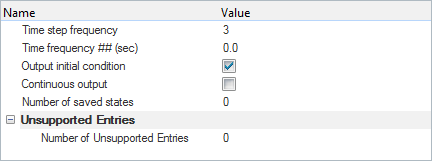
Figure 6.
Specify the Transient Inflow Boundary Conditions and Nodal Initial Conditions
In this step, you will start by creating Multiplier Functions and then specify the transient boundary conditions for both the inlets. Then you will specify the Nodal Initial Conditions for the flow and thermal fields.
Create Multiplier Functions
First, you will create curves for the scaling function to be used for the Multiplier Function type.
-
In the Curve editor dialog, enter the following values for
the curve array.
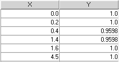
Figure 7. -
In the Curve editor dialog, click on
Small_Inlet in the top-left corner and enter the
following values for the array.
Make sure that the Current curves is showing Small_Inlet.
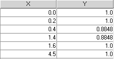
Figure 8. -
Click Update.
Both the curves should be displayed, as shown in the figure below.
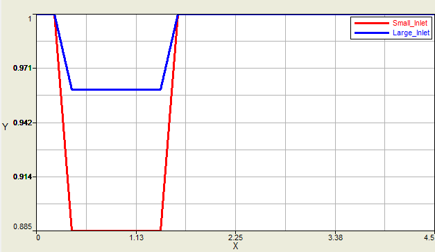 Figure 9. Note: The default color for the curves is grey, which can be changed using the Color option on the bottom left corner of the Curve editor dialog
Next, you will create the Multiplier Functions for both the Inlets.
-
Select the Curve Large_Inlet.
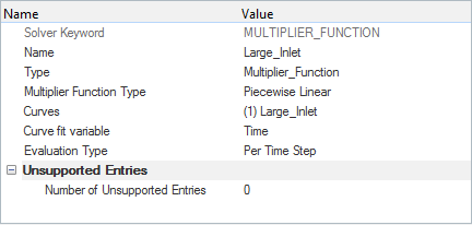
Figure 10.
Specify the Nodal Initial Conditions
In this step, first you will specify the initial values of Pressure, Velocity, Temperature and Eddy Viscosity at all nodes and then Transient BCs for both the inlets.
-
Click on the select file icon in the value field of NIC file, browse to your
working directory, and select the
ConjugateHeatTransfer_Transient.pres.nic file.
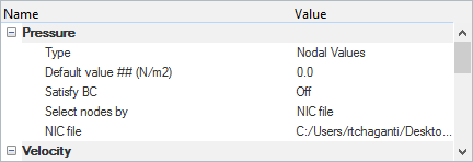
Figure 11.
Specify the Transient Inlet Boundary Conditions
-
Click Large_Inlet. In the Entity Editor, under the Simple Boundary Condition tab,
- Turn On the Show advanced features field.
- Click on the entity collector in the Value field of the Temperature multiplier function and select Large_Inlet. Click OK to close the dialog.
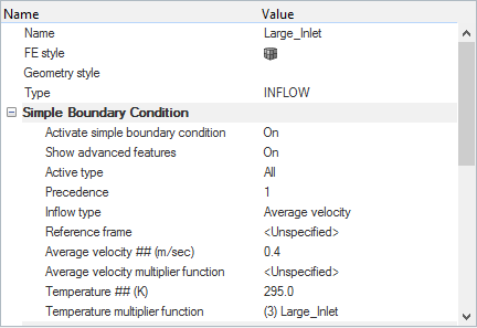
Figure 12.
Compute the Solution
In this step, you will launch AcuSolve directly from HyperMesh and compute the solution.
Run AcuSolve
-
Click on the ACU toolbar.
The Solver job Launcher dialog opens.
-
Leave the remaining options as
default and click Launch to start the solution
process.
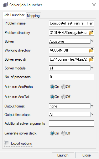
Figure 13.
Post-Process the Results with HyperView
Open HyperView and Load the Model and Results
-
In the Load model and results panel, click
 next
to Load model.
next
to Load model.
Create a Temperature Distribution Animation
-
Click the Isolate Shown icon
 then hold Ctrl and click the
Symmetry and Pipe_Symmetry
components to turn off the display of all components in the graphics window
except the Symmetry and Pipe_Symmetry.
then hold Ctrl and click the
Symmetry and Pipe_Symmetry
components to turn off the display of all components in the graphics window
except the Symmetry and Pipe_Symmetry.
-
Orient the display to the xy-plane by clicking
 on the Standard Views toolbar.
-
Click
 on the Results toolbar to open the Contour panel.
-
In the panel area, under the Display tab, turn off
the Discrete color option.
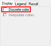
Figure 14. -
On the Animation toolbar, click the Animation Controls icon
 .
.
-
Click the Start/Pause Animation icon
 to play the animation in the graphics area.
Save the Animation
-
On the ImageCapture toolbar, make sure that the Save Image to File option is
On.

-
Click the Capture Graphics Area Video icon
 .
The Save Graphics Area Video As dialog opens.
.
The Save Graphics Area Video As dialog opens.
Summary
In this tutorial, you learned how to set up and run a transient conjugate heat transfer simulation using HyperMesh and AcuSolve. You learned how to specify Nodal Initial Conditions and how to create multiplier functions for setting up the transient boundary conditions. Finally, you used HyperView to create and save an animation of the results of the transient simulation.