ACU-T: 6010 Flow Through Porous Medium
Prerequisites
This tutorial provides the instructions for setting up, solving and viewing results for a simulation of a flow through porous medium. Prior to starting this tutorial, you should have already run through the introductory tutorial, ACU-T: 1000 Basic Flow Set Up, and have a basic understanding of HyperWorks CFD, AcuSolve, and HyperView. To run this simulation, you will need access to a licensed version of HyperWorks CFD and AcuSolve.
Prior to running through this tutorial, copy HyperWorksCFD_tutorial_inputs.zip from <Altair_installation_directory>\hwcfdsolvers\acusolve\win64\model_files\tutorials\AcuSolve to a local directory. Extract ACU-T6010_PorousMedia.hm from HyperWorksCFD_tutorial_inputs.zip.
Problem Description
The problem to be addressed in this tutorial is shown schematically in the figure below. It consists of a cylindrical channel with a porous medium in the flow section. As the flow passes through this section, a pressure drop is observed. In this simulation, an inlet velocity will be assigned to the flow and pressure drop across the porous medium will be calculated. The length of the porous section is 0.06 m and the fluid is an imaginary air-like fluid with a density of 1 kg/m3 and a molecular viscosity of 0.001 kg/m-s. The inlet velocity of the flow is 0.2 m/s.
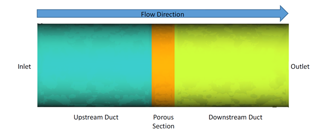
Figure 1.
Start HyperWorks CFD and Open the HyperMesh Database
-
From the Home tools, Files tool group, click the Open Model tool.

Figure 2.The Open File dialog opens.
Validate the Geometry
The Validate tool scans through the entire model, performs checks on the surfaces and solids, and flags any defects in the geometry, such as free edges, closed shells, intersections, duplicates, and slivers.
Figure 3.
Set Up Flow
Set Up the Simulation Parameters and Solver Settings
-
From the Flow ribbon, click the Physics tool.

Figure 4.The Setup dialog opens. -
Under the Physics models setting:
- Set Time marching to Steady.
- Select Laminar as the Turbulence model.
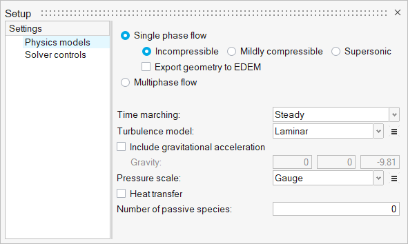
Figure 5. -
Confirm that the Steady update factor and the Steady maximum steps are set to
0.6 and 100,
respectively.
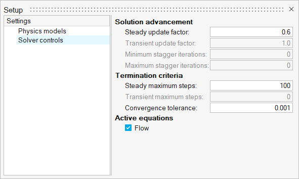
Figure 6.
Assign Material Properties
-
From the Flow ribbon, click the Material tool.

Figure 7. -
Verify that the material Air is assigned to the model's three solids.
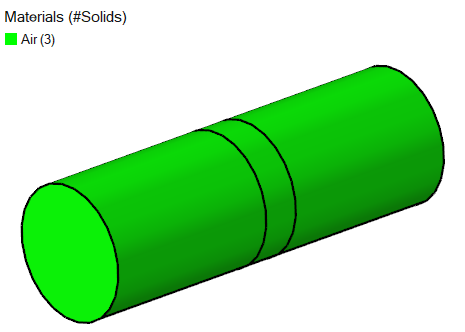
Figure 8.
Define the Porous Medium
-
From the Flow ribbon, Porous
tool group, click the Cartesian Porous Media tool.

Figure 9. -
Select the middle solid on the model.
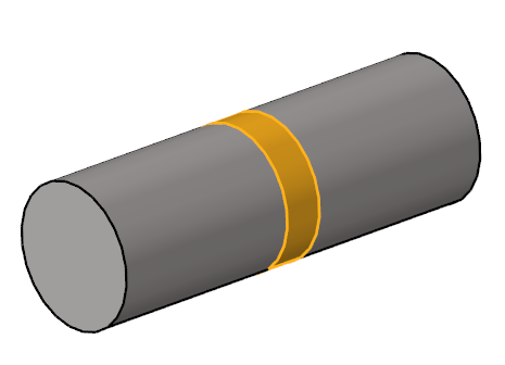
Figure 10. -
In the microdialog, enter the following values for the
coefficients.
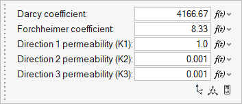
Figure 11. -
In the microdialog, click
 to open the Orient tool then verify that the direction is aligned to the
global x-axis.
to open the Orient tool then verify that the direction is aligned to the
global x-axis.
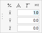
Figure 12. -
On the guide bar, click
 to execute
the command and exit the tool.
to execute
the command and exit the tool.
Assign the Flow Boundary Conditions
-
From the Flow ribbon, click the Constant tool.

Figure 13. -
Select the inlet face.
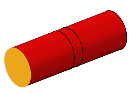 Figure 14.
 -
In the microdialog, set the velocity parameters as
shown below.
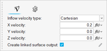
Figure 15. -
On the guide bar, click
to execute
the command and exit the tool.
-
Click the Outlet tool.

Figure 16. -
Select the outlet face.
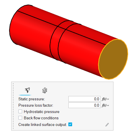
Figure 17. -
Accept the default parameters then click
 on the
guide bar.
on the
guide bar.
Generate the Mesh
-
From the Mesh ribbon, click the Batch tool.

Figure 18.The Meshing Operations dialog opens.Note: If the model has not been validated, you are prompted to create the simulation model before running the batch mesh. -
Accept all other default parameters.
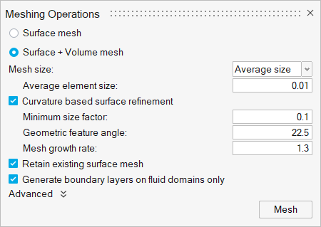
Figure 19.
Run AcuSolve
-
From the Solution ribbon, click the Run tool.

Figure 20. -
Leave the remaining options as default and click
Run to launch AcuSolve.
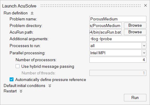
Figure 21.The Run Status dialog opens. Once the run is complete, the status is updated and you can close the dialog.
Post-Process the Results with AcuProbe
As the solution progresses, AcuProbe is launched automatically. AcuProbe can be used to monitor different variables over solution time. In this step, you will plot the residual ratio values and then compute the pressure drop across the porous section.
-
Right-click on Final and select Plot
All.
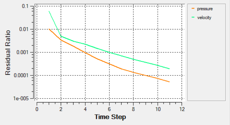
Figure 22. -
Click the User Function icon
 from the toolbar.
The User Function dialog opens.
from the toolbar.
The User Function dialog opens. -
Right-click on pressure and select Copy
name. Paste the value in the Function window after P_In =.
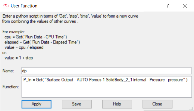
Figure 23. -
On the next line, type value = P_In - P_Out.
Note: The word “value” is case sensitive and should always be in lower case. If you use a capital letter, an error window appears.
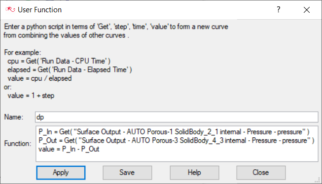
Figure 24. -
Click Apply to display the plot.
Note: You might need to click
 on the toolbar in order to
properly display the plot.
on the toolbar in order to
properly display the plot.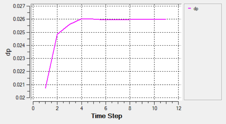
Figure 25.
Summary
In this tutorial, you learned how to set up and solve a flow simulation with porous medium. You started by importing the HyperWorks CFD input database and then you defined the porous medium. Next, you assigned the flow boundary conditions and generated the mesh. Once the solution was computed, you created a plot of the pressure drop across the porous section using AcuProbe.