ACU-T: 3201 Solar Radiation and Thermal Shell Tutorial
This tutorial introduces you to setting up a CFD simulation involving solar radiation and thermal shells using AcuSolve and HyperWorks CFD. Prior to starting this tutorial, you should have already run through the introductory tutorial, ACU-T: 1000 Basic Flow Set Up, and have a basic understanding of HyperWorks CFD, AcuSolve, and HyperView. To run this simulation, you will need access to a licensed version of HyperWorks CFD and AcuSolve.
Prior to running through this tutorial, copy HyperWorksCFD_tutorial_inputs.zip from <Altair_installation_directory>\hwcfdsolvers\acusolve\win64\model_files\tutorials\AcuSolve to a local directory. Extract ACU-T3201_Atrium.x_t and SolarLoad.dat from HyperWorksCFD_tutorial_inputs.zip.
Problem Description

Figure 1.
Solar Radiation Parameters
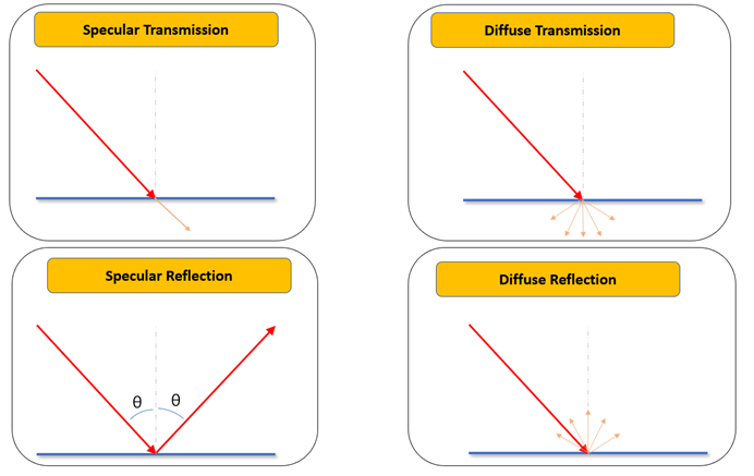
Figure 2.
- Specular transmissivity
- Diffuse transmissivity
- Specular reflectivity
- Diffuse reflectivity
- Absorptivity
- Angle of incidence
For the solar radiative heat fluxes to be computed, a solar radiation surface needs to be defined on that given surface.
In this tutorial, the solar flux loading is given in the form of a data file which was generated using the acuSflux script available in AcuSolve. The script can be used to generate a data file with a four-column array of solar flux vector data values. The piecewise linear type is used in this tutorial to emulate the pattern of sunrise to sunset over the atrium.
For example, to generate the solar load data file for a location with known geological coordinates, enter the following command in the AcuSolve Command Prompt: acuSflux -time "dec-3-2019 11:00:00" -tinc 1800 -nts 25 -lat 42.6064 -lon -83.1498 -ndir "1,0,0" -udir "0,0,1"
- time
- The start time in GMT (ex: “dec-3-2019 21:00:00”)
- tinc
- The time increment in seconds
- nts
- Number of discrete time steps
- lat
- Latitude coordinates of the location in degrees North (ex: 45.112 or -37.56 (equal to 37.56 S))
- lon
- Longitude coordinates of the location in degrees East (ex: 86.26 or -54.84 (equal to 54.84 W))
- ndir
- The north direction unit vector in model coordinates (should be enclosed in double quotes) (ex: “0,1,0”)
- udir
- The upward direction unit vector in model coordinates (should be enclosed in double quotes) (ex: “0,1,0”)
Thermal Shell Modeling
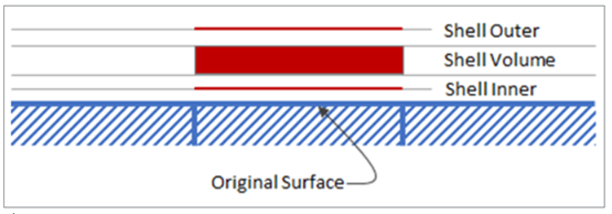
Figure 3.
When defining a thermal shell on a surface, two sets of boundary conditions are needed. One for the Primary Wall surface i.e. Shell Inner and one for the Shell Outer Wall surface. In this tutorial, a solar radiation surface will be defined on the outer shell surface so that it receives solar heat flux, whereas the inner shell surface will be modeled as a default wall.
Start HyperWorks CFD and Create the HyperMesh Model Database
-
Create a new .hm database in
one of the following ways:
- From the menu bar, click .
- From the Home tools, Files tool group, click the Save As tool.
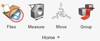
Figure 4.
Import and Validate the Geometry
Import the Geometry
-
In the Geometry Import Options dialog, leave all the
default options unchanged then click Import.
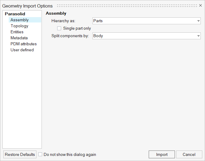
Figure 5.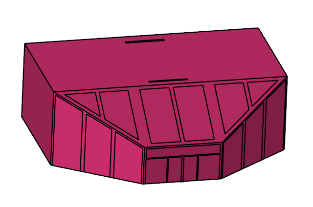
Figure 6.The model contains an atrium with glass panes supported by an aluminum frame in the front. Air enters from the opening on the roof in the front and exits through the outlet in the rear.
Validate the Geometry
-
From the Geometry ribbon, click the Validate tool.

Figure 7.The Validate tool scans through the entire model, performs checks on the surfaces and solids, and flags any defects in the geometry, such as free edges, closed shells, intersections, duplicates, and slivers.The current model doesn’t have any of the issues mentioned above. Alternatively, if any issues are found, they are indicated by the number in the brackets adjacent to the tool name.
Observe that a blue check mark appears on the top-left corner of the Validate icon. This indicates that the tool found no issues with the geometry model.
Figure 8.
Set Up Flow
Set Up the Simulation Parameters and Solver Settings
-
From the Flow ribbon, click the Physics tool.

Figure 9.The Setup dialog opens. -
Under the Physics models setting:
- Set Time marching to Transient.
- Set the Time step size to 1 and the Final time to 30.
- Set the Turbulence model to Laminar.
- Activate the Heat transfer checkbox.
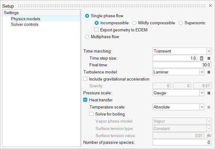
Figure 10. -
Click the Solver controls setting and set the Maximum
stagger iterations to 3.
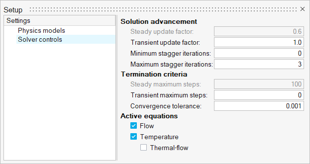
Figure 11.
Assign Material Properties
-
From the Flow ribbon, click the Material tool.

Figure 12. -
Verify that Air is assigned as the material for the fluid domain.
The legend in the top-left corner of the modeling window lists all the material models assigned to the current model.Since this model has a single volume, by default air is assigned as the material for the fluid domain.
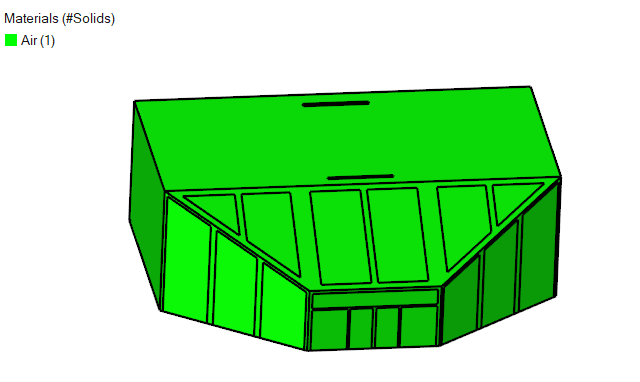
Figure 13. -
On the guide bar, click
 to execute
the command and exit the tool.
to execute
the command and exit the tool.
Define Thin Solids
In this simulation, you will model the aluminum frames as a thin solid.
-
From the Flow ribbon, click the Thin tool.

Figure 14. -
In the modeling window, select the four surfaces
highlighted in the image below.
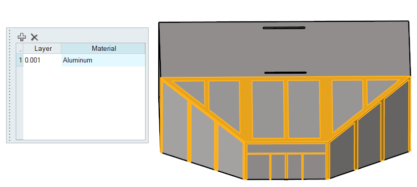
Figure 15. -
On the guide bar, verify that the number of Parent
Surfaces selected is 4 then click
 to execute the
command.
Once the command is executed, the legend should be updated accordingly to reflect the changes.
to execute the
command.
Once the command is executed, the legend should be updated accordingly to reflect the changes.
Define Flow Boundary Conditions
-
From the Flow ribbon, click the Constant tool.

Figure 16. -
In the modeling window, click the inlet surface
highlighted in the figure below.
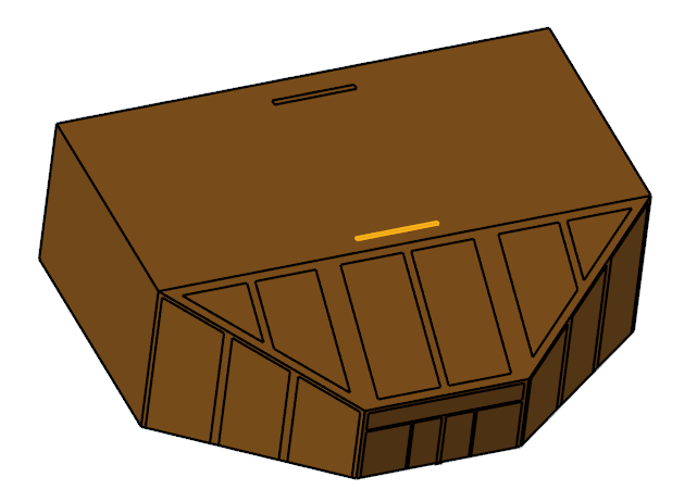
Figure 17. -
In the microdialog, enter the values shown below.
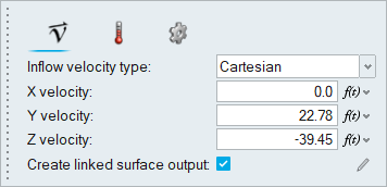
Figure 18. -
Click the Temperature icon and enter a value of
295.35 K.
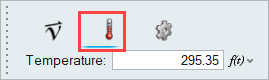
Figure 19. -
Click on the guide bar to execute the changes.
-
Click the Outlet tool.

Figure 20. -
Select the surface highlighted in the figure below then click on the
guide bar.
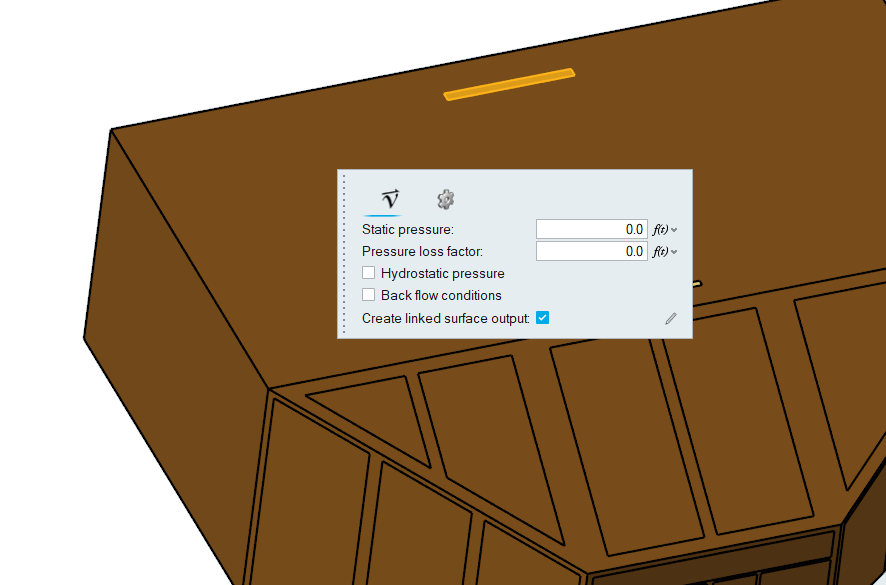
Figure 21. -
Click the No Slip tool.

Figure 22. -
Select all three wall surfaces of the atrium, the roof, and the front glass
walls.
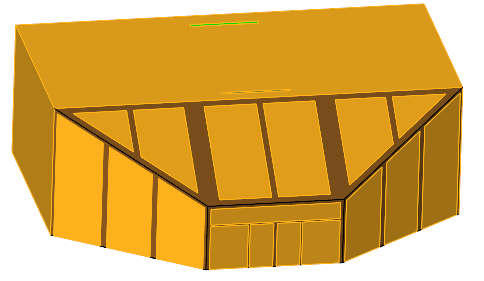
Figure 23. Front-Side of the Model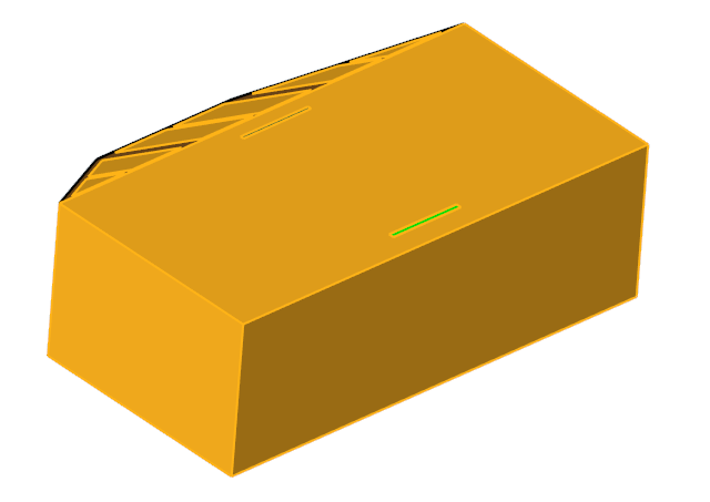
Figure 24. Back-Side of the ModelIn total, 21 surfaces should be selected.
-
In the microdialog, enter the values shown in the
figure below.
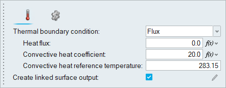
Figure 25. -
Click
 . In the
new microdialog that appears, set the Nodal Output
frequency to 1.
. In the
new microdialog that appears, set the Nodal Output
frequency to 1.
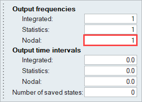
Figure 26. -
On the guide bar, click
 to execute the command and remain in the
tool.
to execute the command and remain in the
tool.
-
Select all the thin solid surfaces using the window selection method.
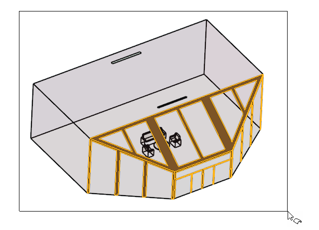
Figure 27. -
In the microdialog, enter the values shown in the
figure below.
Figure 28. -
Click . In the
new microdialog that appears, set the Nodal Output
frequency to 1.
-
On the guide bar, verify that the number of Thin Solids
selected is 4 and the Direction is set to Away from Parent
Surface, then click .
-
From the Boundaries legend, right-click on Default Wall
and select Isolate.
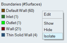
Figure 29. -
Select all the surfaces except the aluminum frame, as highlighted in the figure
below.
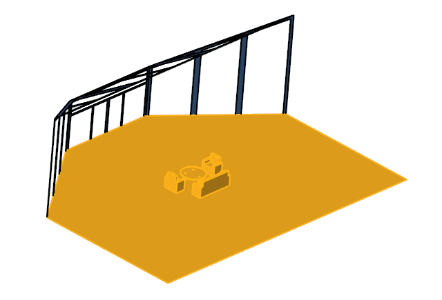
Figure 30. -
In the microdialog, enter the values shown in the
figure below.
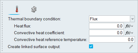
Figure 31. -
Click . In the
new microdialog that appears, set the Nodal Output
frequency to 1.
-
Click on the
guide bar.
The updated Boundaries legend should look similar to the one shown below.
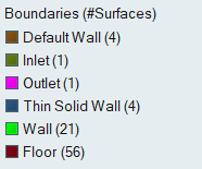
Figure 32.
Set Up Solar Radiation
Set Up the Solar Radiation Parameters
-
From the Radiation ribbon, Solar Radiation tools, click the Physics tool.

Figure 33. -
Click
 to load
the solar flux input from a file.
to load
the solar flux input from a file.
-
Click Open.
The plot in the dialog should look like the one shown in the figure below.
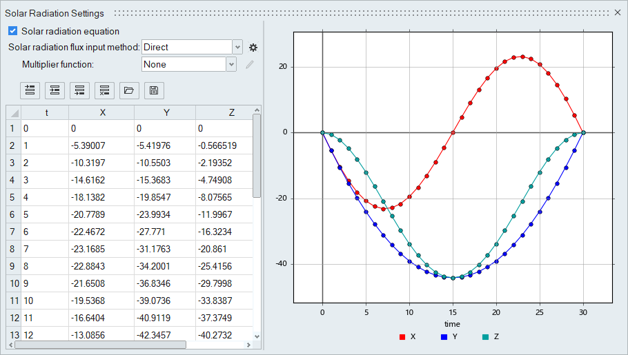
Figure 34.
Define the Solar Radiation Models
-
From the Radiation ribbon, Solar Radiation tools, click the Model tool.

Figure 35. -
In the Solar radiation model library, click
 to add a new
solar radiation model.
to add a new
solar radiation model.
-
Similarly, create the other models and enter the values as shown in the figure
below.
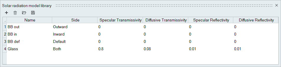
Figure 36.
Assign the Solar Radiation Models
-
From the Radiation ribbon, click the
Surface tool.

Figure 37. -
Select the three wall surfaces, the inlet, and the roof surface, as highlighted
in the figures below.
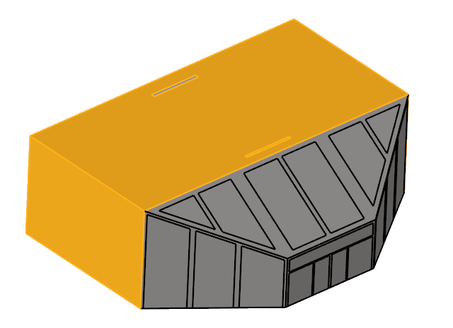
Figure 38. Front-Side of the Model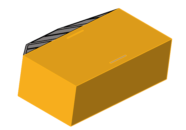
Figure 39. Back-Side of the Model -
In the microdialog, set the Solar radiation model to
BB out then click on the
guide bar.
-
Select all the glass surfaces shown in the figure below, assign the
Glass model to them, then click on the
guide bar.
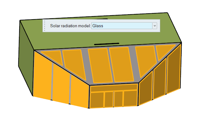
Figure 40. -
Rotate the model and select the floor surface. In the microdialog, assign the BB in model
then click on the
guide bar.
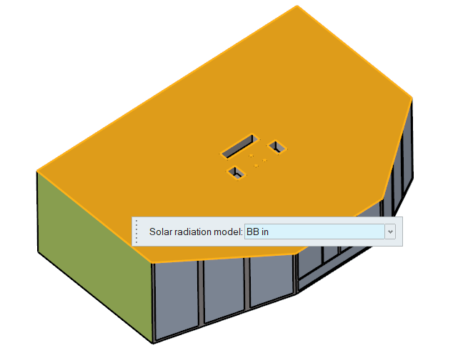
Figure 41. -
Select the surfaces of the couch, table, and chairs, assign the BB
def model to them, then click on the
guide bar.
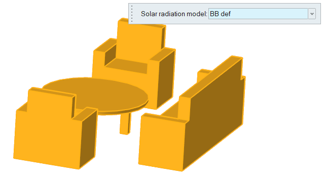
Figure 42. -
Using the window selection method, select the four thin solid surfaces and
assign the BB out model to them.
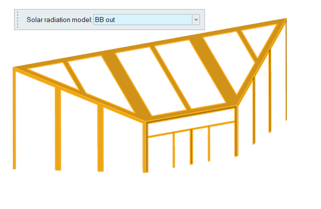
Figure 43. -
On the guide bar, verify that the Direction is set to
Away from Parent Surface then click
 to execute
the changes.
to execute
the changes.
Generate the Mesh
In this step, you will define the mesh controls and then generate the mesh.
Define the Surface Mesh Controls
-
From the Mesh ribbon, click the Surface tool.

Figure 44. -
In the microdialog, set the Average element size to
0.15 and the Mesh growth rate to
1.0.
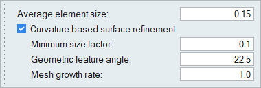
Figure 45. -
On the guide bar, click
to execute
the command and exit the tool.
Generate the Mesh
-
From the Mesh ribbon, click the Batch tool.

Figure 46.
Compute the Solution
Define the Nodal Output Frequency
-
From the Solution ribbon, click the Field tool.

Figure 47. -
Set the Time step interval to 1.
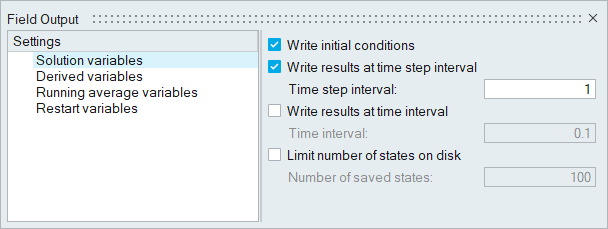
Figure 48.
Define the Nodal Initial Conditions and Compute the Solution
-
From the Solution ribbon, click the Run tool.

Figure 49. -
Verify that all the values are set as shown in the figure below.
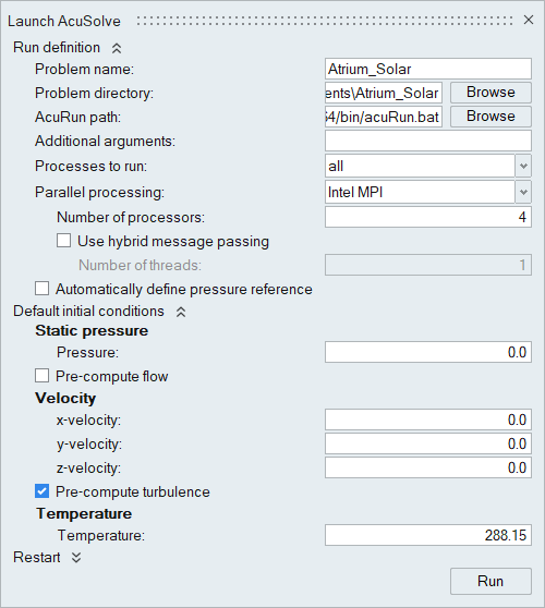
Figure 50. -
In the dialog, right-click on the AcuSolve run and
select View log file.
Once the run is complete, a summary of the solution process is shown in the log file.
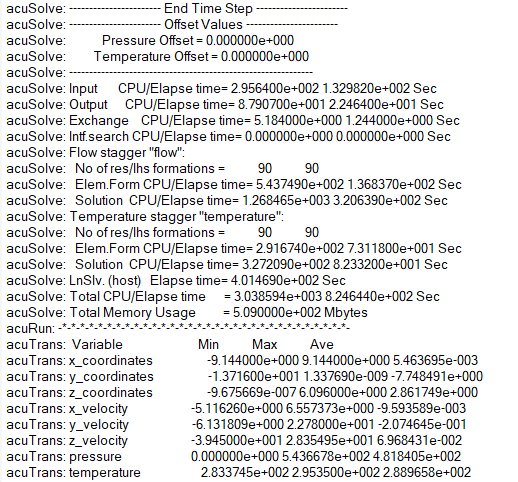
Figure 51.
Post-Process the Results with HyperView
In this step, you will create an animation of solar heat flux and temperature over run time.
Open HyperView and Load the Model and Results
-
In the Load model and results panel, click
 next
to Load model.
next
to Load model.
-
In the Reader Options dialog, set the Reader to
AcuSolve Result Reader and the Extended nodal output
option to Yes then click OK.
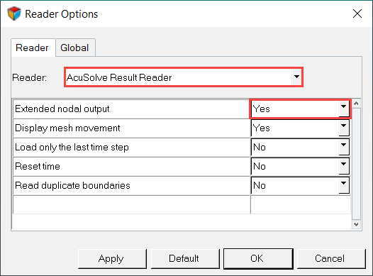
Figure 52.
Create an Animation of Temperature Contour
In this step, you will start by creating an expression for plotting the temperature values in Fahrenheit units. Then, you will create an animation of the magnitude of temperature on the floor and the thin solid wall surfaces.
-
Complete the expression by entering the remaining portion of the formula as
shown in the figure below.
Here the term ‘R1.S10’ corresponds to the Temperature (scalar) variable in Kelvin. Variables can be inserted in the expression by selecting the required variable under Table option and then clicking Insert. The actual ID for the scalar variable might be different for your simulation.
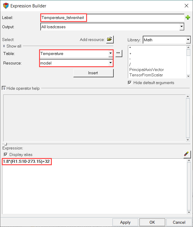
Figure 53. -
In the Results Browser, expand the list of
Components. Turn off the display of all the
components except Floor - Output and Thin
Solid Wall - Dynamic.
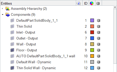
Figure 54. -
Click
 on the Results toolbar to open the Contour panel.
-
In the panel area, under the Display tab, turn off
the Discrete color option.
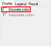
Figure 55. -
Click
 on the Animation toolbar to play the temperature
animation.
on the Animation toolbar to play the temperature
animation.
-
Click the Animation Controls icon
 . In the panel area, set the Max
Frame Rate to 5 Frames/Sec by dragging the slider.
. In the panel area, set the Max
Frame Rate to 5 Frames/Sec by dragging the slider.
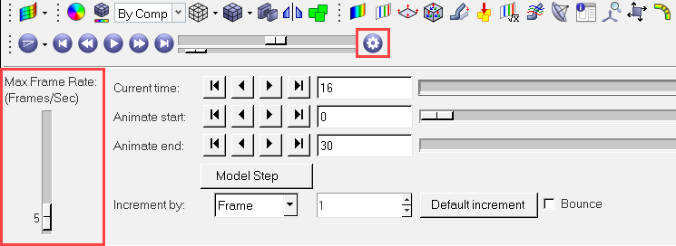
Figure 56.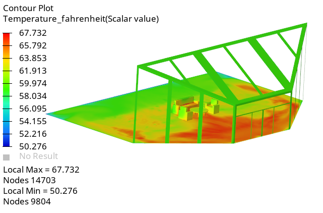
Figure 57.
Create an Animation of Solar Heat Flux
-
Click
on the Results toolbar to open the Contour panel.
-
Click Apply.
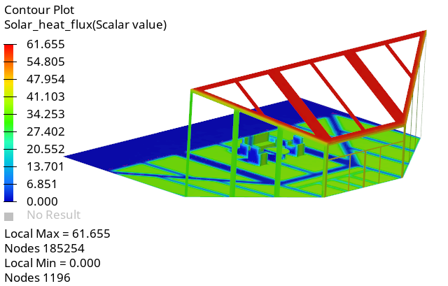
Figure 58. -
On the ImageCapture toolbar, click on the Capture Graphics Area
Video icon
 .
.
Summary
In this tutorial, you learned how to set up and solve a CFD analysis involving solar radiation. You started by importing a geometry model into HyperWorks CFD and setting up the simulation parameters and boundary conditions. Once you computed the solution, you post-processed the results using HyperView. Also, you learned how to create expressions in HyperView so that you can build plots of derived results.