Plot Run Time Data
Use the Plot tool to track converged and derived solution behavior in real time.
Open .log Files and View Plots
-
Open a .log file in the Plot
tool in the following ways:
- From the Solution ribbon, click the
Plot tool.

Figure 1.In the Plot Utility dialog, click
 then browse
and select a file.
then browse
and select a file. - From the Run Status dialog, right-click on an AcuSolve run and select Plot time history from the context menu.
- From the Solution ribbon, click the
Plot tool.
-
Double-click on an option in the library to view the plot in a new tab.
Convergence plots for residual ratios and solution ratios are available by default.
If AcuSolve is still running, the plots update in real time to track the solution progress.
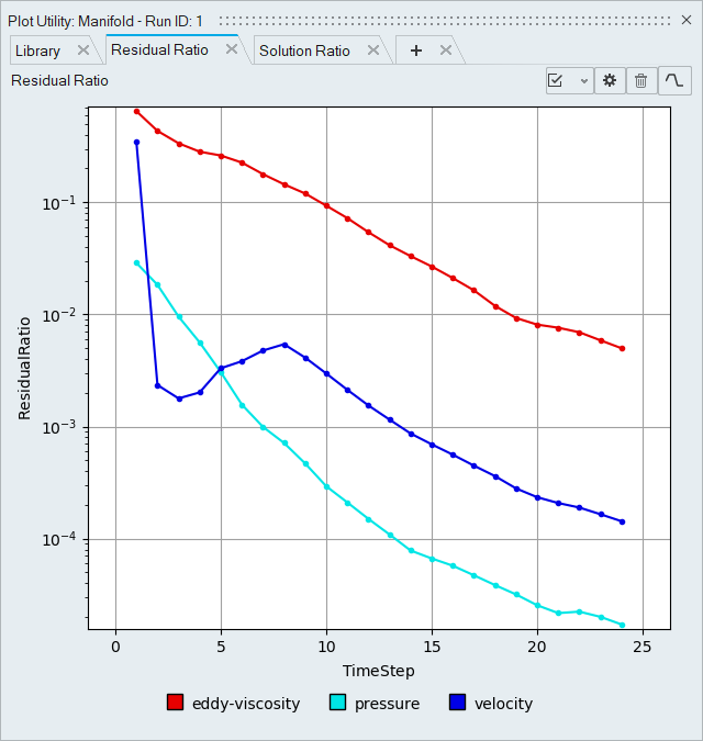
Figure 2.
Tip:
- Left-click and draw a window in the plot to zoom in on the defined area. Right-click to return to the default view.
- Click
 to change the
scale from linear to logarithmic.
to change the
scale from linear to logarithmic.
Create Plots
-
From the Solution ribbon, click the
Plot tool.
Figure 3.The Plot Utility dialog opens. -
Click
 in the tab area to create a new
plot.
in the tab area to create a new
plot.
-
Define the y-axis.
-
For surface output and statistics, select a variable
sub-category.
Direction orientated variables, such as velocity, momentum, and shear stress require you to select a coordinate direction. Click below the y-axis definition
to plot multiple directions.
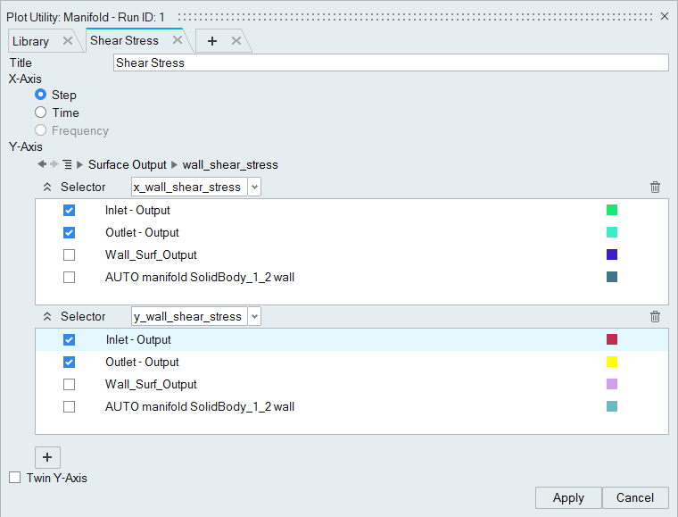
Figure 4.Tip: Activate Twin Y-Axis to define a second set of y-axis variables. -
For surface output and statistics, select a variable
sub-category.
Edit Plots
-
From the Solution ribbon, click the
Plot tool.
Figure 5.The Plot Utility dialog opens. -
From either the plot library or an individual plot tab, click
 .
.
Delete Plots
-
From the Solution ribbon, click the
Plot tool.
Figure 6.The Plot Utility dialog opens. -
Click
 .
.
Export Plots
-
From the Solution ribbon, click the
Plot tool.
Figure 7.The Plot Utility dialog opens. -
From the plot library, click
 to save the entire plot
workspace.
to save the entire plot
workspace.
-
From a plot tab, click
 then select
Export to save the individual plot.
then select
Export to save the individual plot.