Cell Parameters Output
The different cell parameters and their output files are described using examples.
Figure 1 shows an example of a typical urban configuration.
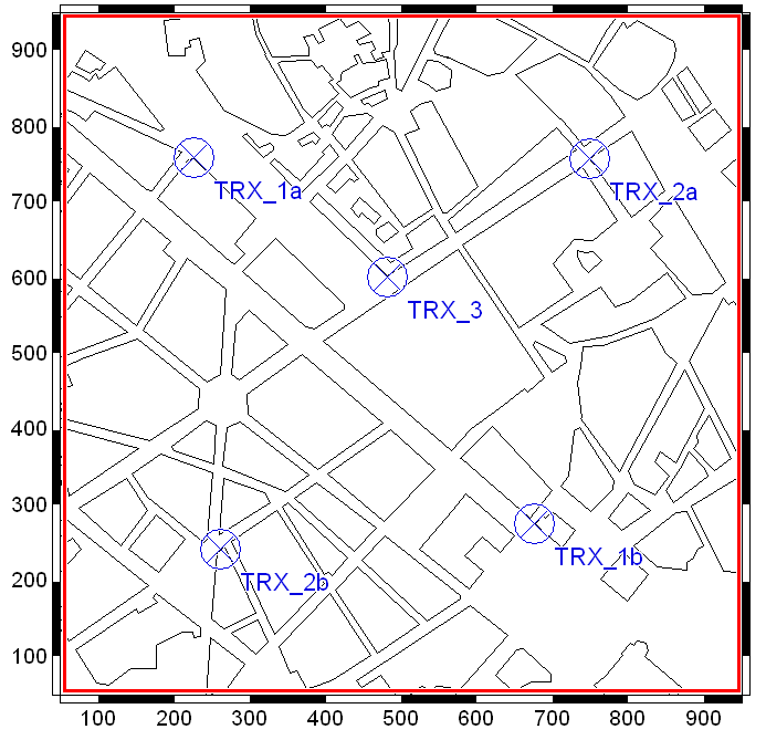
Figure 1. Typical urban configuration for ProMan.
The base stations TRX_1a and TRX_1b use the same channel #50, TRX_2a and TRX_2b use the same channel #60 and TRX_3 uses channel #70. All base stations have the same transmit power.
Co-Channel Interference (CCI) (.fpc)
- The individual CCI computation:
This computation is done for each channel for the whole prediction area. The CCI is only computed if two base stations use the same channel. The result files are named: output-filename_Cxx.fpc, where “xx” is the channel number.
Figure 2 shows the results for the two transmitter pairs. The scale is the same as that used in Figure 3.
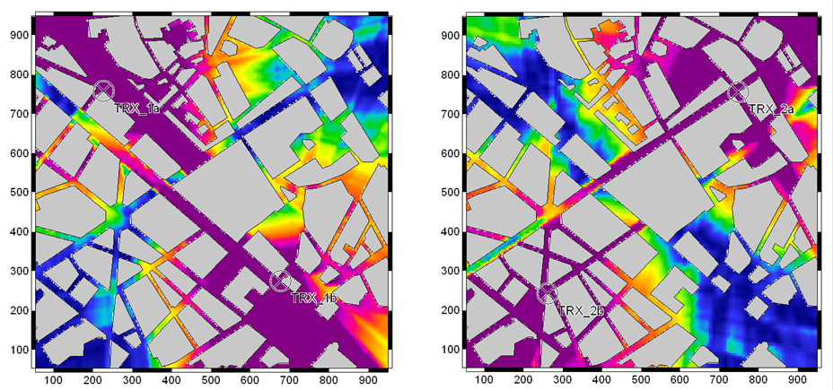
Figure 2. Individual CCI computation: TRX 1a and 1b (left), and TRX 2a and 2b (right). - The total CCI computation:
The CCI is computed for all channels respectively where the individual channel is best server. The result files are named output-filename.fpc. shows an example of a .fpc file:
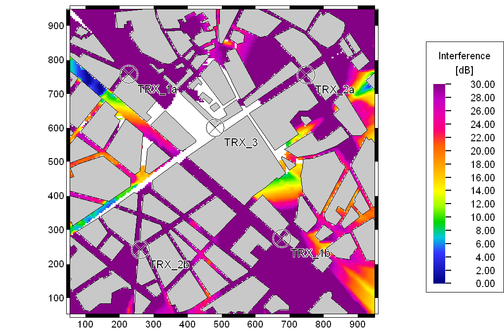
Figure 3. Example of a total CCI computation result.
The total CCI is always computed in the areas where the individual channel is the best server channel.
Best Server (.fpb)
A best server plot shows the channel number of the channel that provides the maximum received power at the individual point. Figure 4 shows the result.
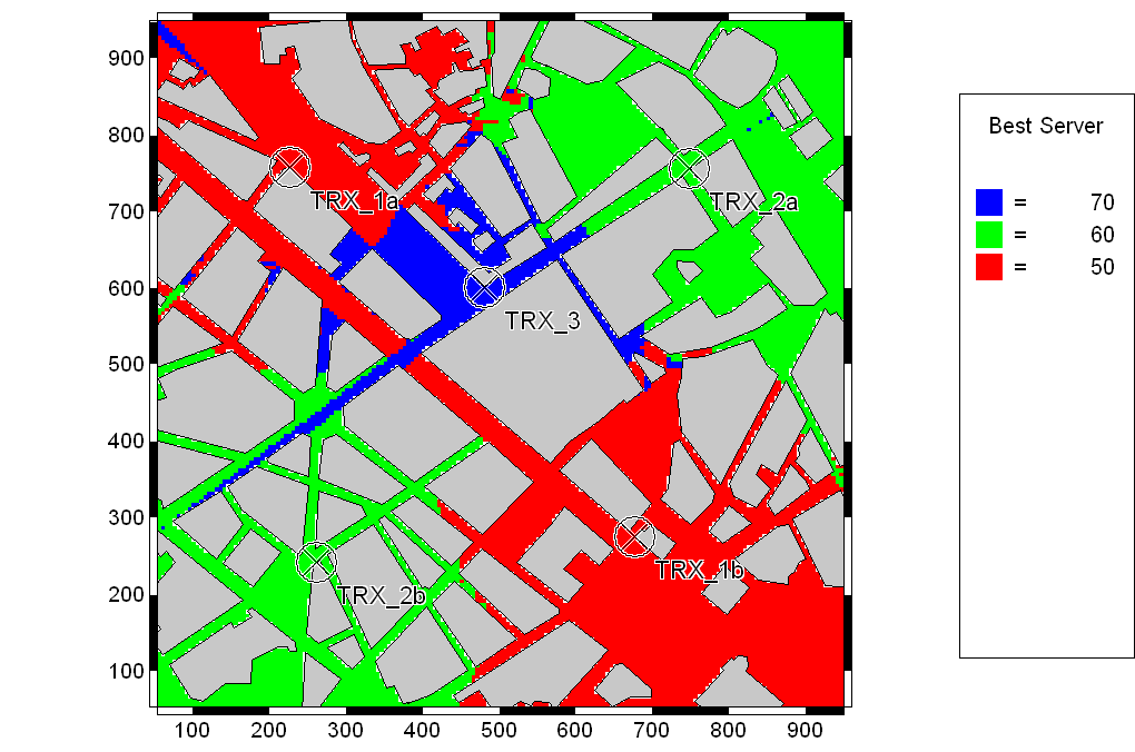
Figure 4. Example of a best server plot.
Maximum Value (.fpm)
For each receiver pixel a prediction of each base station is computed. The maximum value of the received power in dBm at each pixel is chosen and displayed.
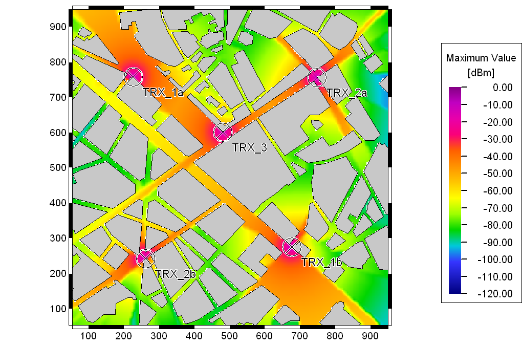
Figure 5. Example of a prediction of the maximum value.
Superpose transmitters (.fpa For Received Power In [dBm] and .fpe For Field Strength In [dBµV/m])
For each channel the prediction of all base stations with this channel number are accumulated and the result is written in a file for each channel (the file name gets an extension, for example, _C60 for channel 60).
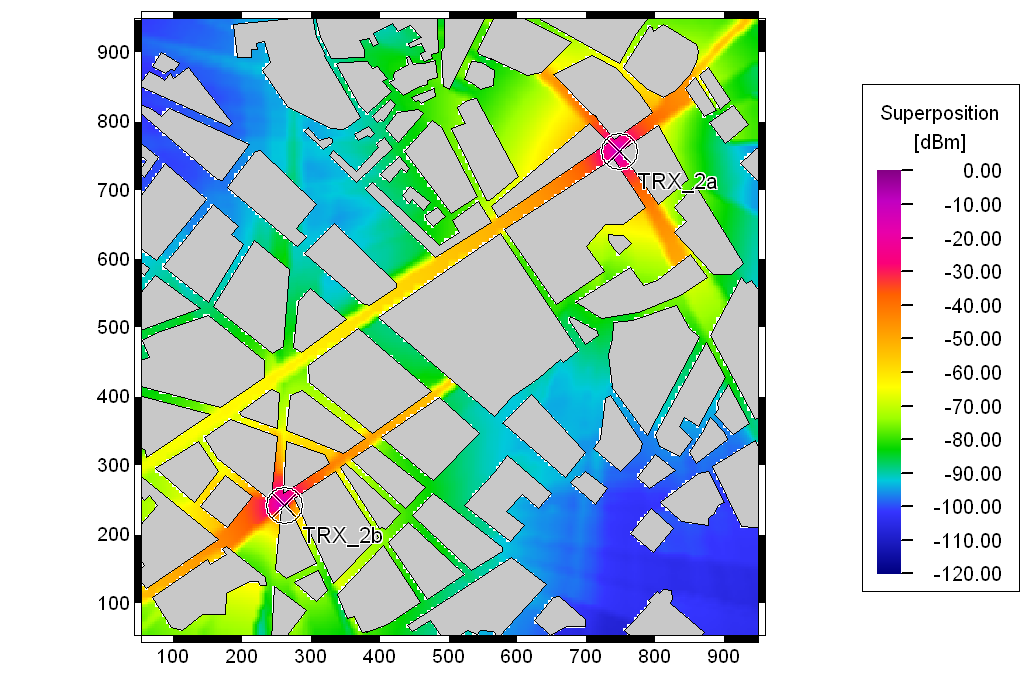
Figure 6. Prediction plot for channel 60 by superposing two transmitters.
Coverage Degree (Number of Channels Higher Than Threshold) (.fpn)
For every prediction pixel, the number of base stations where the predicted received power is above a user-defined threshold is computed. This threshold can be changed in the prediction parameter section of the ProMan. The result reflects the coverage degree in the individual positions.
Figure 7 shows the coverage degree result. It is visible that in some areas a bad coverage (degree of 0) is achieved.
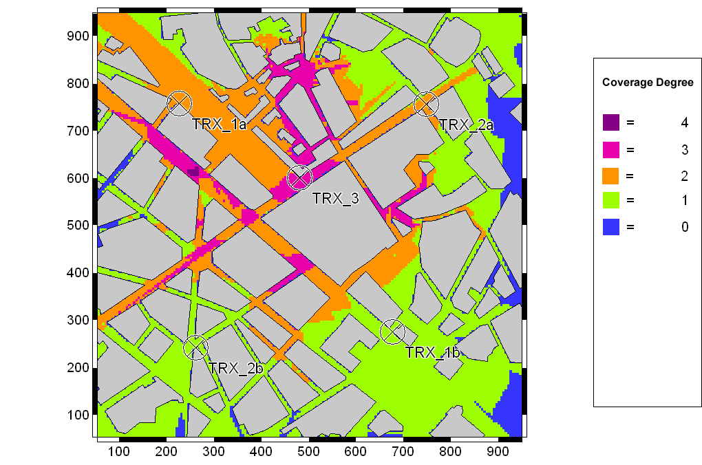
Figure 7. Prediction plot for the degree of coverage.