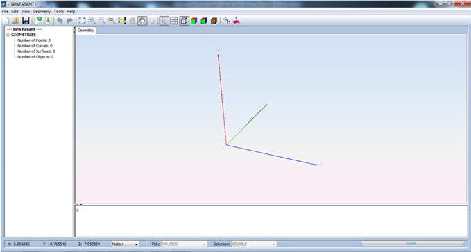
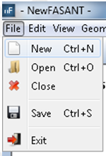
Create a new newFASANT project. To do this, select the
File → New option (alternatively, the press Ctrl+N).
Figure 2. File menu
Step 3
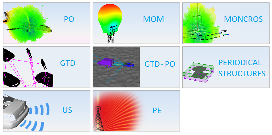
After selecting the New option, a list of the available modules is presented. The
user needs to select a module from the available module list. Select MONCROS for
this training example.
Figure 3. Module selection screen
Step 4
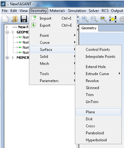
Select the Geometry → Surface → Plane option.\
Figure 4. Geometry → Surface menu
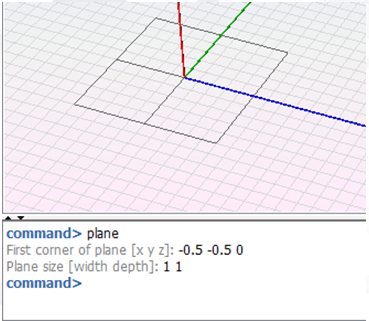
Step 5
The command line panel requires some parameters at this point. Enter “-0.5 -0.5 0” as
the first parameter and “1 1” as the second parameter so we create a 1x1 plane
centered at the origin.
Figure 5. Creating a 1x1 plane
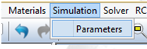
Step 6
Select the simulation parameters option.
Figure 6. Simulation menu
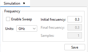
Step 7
Select a frequency of 0.3 GHz (default options) and press Save.
Figure 7. Simulation options
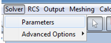
Step 8
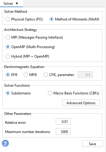
Select the Solver → Parameters option:
Figure 8. Solver menu
Figure 9. Solver parameters
Check the default parameters as the follow figure.
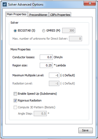
Click on the “Advanced Options” button to set up other solver parameters:
Figure 10. Advanced parameters of solver, 'Main Properties' tab
Save the values for the advanced parameters of the solver.
Step 9
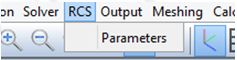
Select the RCS → Parameters option:
Figure 11. RCS menu
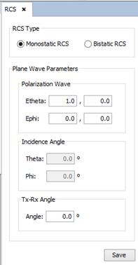
Step 10
Select Monostatic RCS and leave the default parameters. Press the Save button.
Figure 12. RCS parameters
Step 11
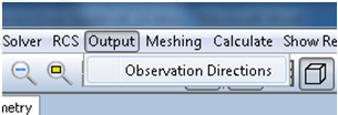
Select Output → Observation directions.
Figure 13. Output menu
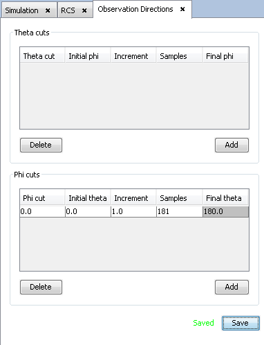
Step 12
Leave the default observation directions (0.0 phi cut with theta angle varying
between 0.0 and 180.0 using 181 samples).
Figure 14. Observation directions options
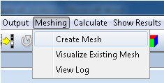
Step 13
Before running the simulation, select the Meshing → Create Mesh option.
Figure 15. Meshing menu
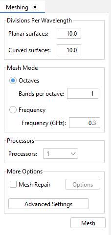
Step 14
Set 10 divisions on planar and curved surfaces, set Processors to 1 and the default
number of bands per octave. Press the Mesh button.
Figure 16. Meshing options
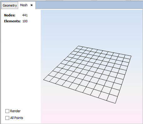
Figure 17. Mesh visualization
Step 15
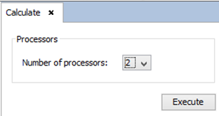
Select Calculate → Execute and set the number of desired processors to run the
simulation. Press the Execute button to start the calculation.
Figure 18. Calculate options
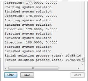
Figure 19. Process Log showing the progress of the calculation
Step 16
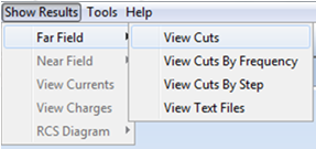
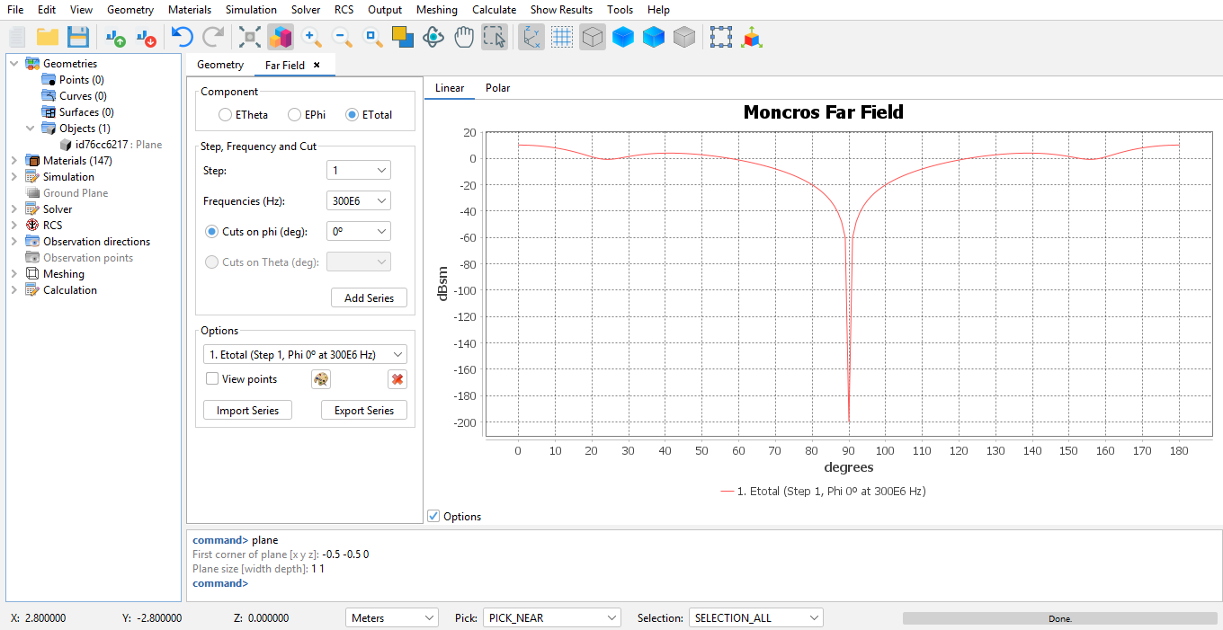
When the simulation finishes (the progress bar on the bottom-left corner displays
“Done”), we are able to see the results. Select the Show Results → Far Field → View
cuts option to show the RCS plot.
Figure 20. Show Results → Far Field menu
Figure 21. RCS graphic
Step 17
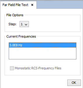
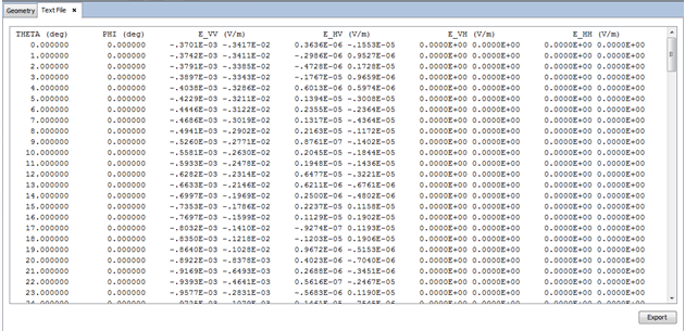
Select Show Results → Far Field → View Text Files to show the RCS data in text
format.
Figure 22. Show Results → Far Field menu
Select the desired frequency and press OK.