In this tutorial, you will learn how to convert results simulation run into file
formats that can be used for fatigue analysis (using a tool like NCode) and how to write a
fatigue analysis file from the MotionView animation
window.
The following functionalities are used in this tutorial: Fatigue Prep, Flex File
Gen, and build plots.
Fatigue Prep
Access this feature from the menu bar by
clicking Flex Tools > Fatigue Prep.
Figure 1.
This panel translates the files listed in Table 1:
Table 1.
Original Format
Translated Format
Altair .H3D flexbody (modal content)
Ncode .FES/.ASC
Ncode .DAC
Altair .ABF
ADAMS .RES (modal participation factors)
Ncode .DAC
ADAMS .REQ files (loads information)
Ncode .DAC
Altair .PLT
Ncode .DAC
ADAMS .REQ files (loads information)
MTS .RPC
Flex File Gen
Access this feature from the menu bar by
clicking Flex Tools > Flex File Gen.
Figure 2.
The Flex File Gen feature allows you to create an
.flx file using the Flex File Gen tool. This file
references a .gra file (rigid body graphics), a
.res file (flex and rigid body results), and
.h3d files (flexbody graphics). These files are
required to animate ADAMS results that contain
flexbodies. The .flx file can be loaded directly into
the animation window.
build plots
From the HyperGraph client, access this
feature by clicking the (build plot) icon.
The Build Plots panel constructs multiple curves and plots from a
single data file. Curves can be overlaid in a single window or each curve
can be assigned to a new window. Individual curves are edited using the
Define Curves panel.
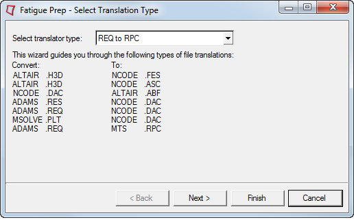
Use the Fatigue Prep Wizard
In this step, you will use the Fatigue Prep Wizard to convert an H3D file into an FES
file.
Start a new MotionView session.
Select the MBD Model window.
From the menu bar, click Flex Tools > Fatigue Prep.
Figure 3. Fatigue Prep Wizard
The form shows the set of file translations that are possible using the
Fatigue Prep Wizard.
From the drop-down menu, choose H3D to FES. Then click
Next.
Specify the H3D file sla_flex.h3d, located in the
mbd_modeling\durability_fatigue folder.
Specify the FES file as <working
directory>\sla_flex_left.fes.
Figure 4. Fatigue Prep Wizard
Click Finish.
The Altair flexible body pre-processor is launched and the FES file is
created in your <working directory>.
Using the Fatigue
Prep wizard, you can convert your results files to
.fes, .asc or
.dac files. You can use these files for fatigue and
durability analysis in Ncode’s FE-Fatigue software.
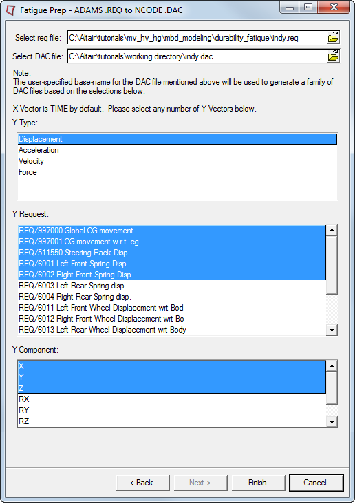
Convert ADAMS results from REQ to DAC
In this step, you will convert the results of an ADAMS
run to DAC files using the Fatigue Prep translator.
Start a new MotionView session.
Select the MBD Model window.
From the menu bar, click Flex Tools > Fatigue Prep.
From the drop-down menu, choose REQ to DAC. Then click
Next.
For Select req file, click the file browser button and specify the req as
indy.req, located in the
durability_fatigue folder.
Note: The DAC file format does not support unequal time steps since only
frequency is specified, not each time step. Therefore your REQ file needs to
have equal output time steps.
For Select DAC file, click the file browser button and specify
indy.dac as the output file name in
<working directory>.
For Y Type, choose Displacement.
The Y request and Y components will automatically populate the next
fields.
Select the first five Y requests and the first three
Y components.
Figure 5. REQ to DAC translation
Note: You can select any number of Y requests and Y components for REQ2DAC
conversion.
Click Finish.
The message 'Translation complete' is displayed on the screen. MotionSolve generates 15 DAC files for each combination
selected.
Click Cancel and close the window.
Change the application to HyperGraph 2D.
From the Build Plots panel, load the file
indy_D_997000_X.dac from your <working
directory>.
Note: In this filename, D represents Displacement, 9970000 represents the
request number, and X represents the component. This is how you get the
information about the DAC file you are plotting.
To see the plot, click Apply.
Note: You can plot the results from the original REQ file for comparison.
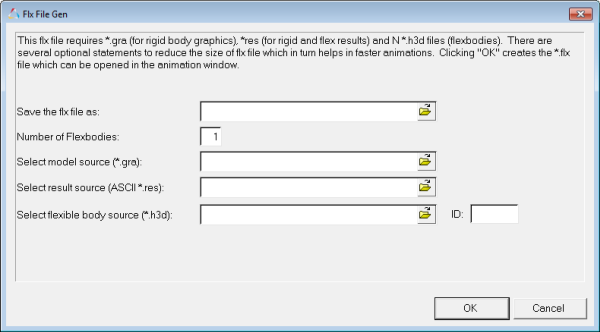
Use the Flex File Tool
Now you will learn to use the Flex File tool.
Start a new MotionView session.
From the menu bar, click Flex Tools > Flex File Gen.
This displays the Flex File Generator dialog. The
dialog lists the files you will need for the conversion.
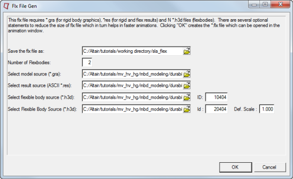
Use Save the *flx file as and specify the destination of
the file as <working-dir>\sla_flex.
In the Number of Flexbodies field, enter 2 (the model
includes two lower control arms as flexible bodies).
Use the Select model source (*.gra) file browser to
select the sla_flex.gra file from the
durability_fatigue folder.
Use the Select result source (ASCII *.res) file browser
to select sla_flex.res file from the
durability_fatigue folder.
Use the first Select flexible body source (*.h3d) file
browser to select sla_flex.h3d file from the
durability_fatigue folder.
Use the second Select flexible body source (*.h3d) file
browser to select sla_flex_m.h3d file from the
durability_fatigue folder.
Under ID, enter 10404 and 20404
for the two H3Ds respectively.
These values should correspond to the actual IDs of the flexible bodies in the
ADM input deck of the ADAMS solver.
The
deformation of these flexible bodies during animation can be scaled using
the Def. Scale field. In this case, accept the default value of
1.000.
Figure 6.
Click OK.
This will launch the translator and create the FLX file in the
destination directory.
In the Select application list, choose TextView.
On the Standard toolbar, click (Open Document).
Open the file sla_flex.flx.
You should see the following contents of the file: Figure 7.
Note:
To load transients results for selected time intervals check the
Optional flx statements check-box to enter
the Start Time, End Time and Increment.
To load selected mode shapes from modal animation files for models with
one or more flexible bodies, check the Optional flx
statements for linear analysis check-box to enter the
Start Mode and End Mode.
Additional statements are inserted in the FLX file reflecting the above
mentioned parameters.
View the Fatigue Results
In this step you will view the Fatigue results in the animation window.
Use the Select application drop-down menu, choose HyperView.
On the Standard toolbar, click
(Open Model).
Use the Load model file browser to select the file
sla_flex.flx.
The Load result field will automatically populate with the same file
name.
Click Apply.
You can use the (Start/Pause Animation) button
to animate the model. Observe the model, which is a combination of rigid
multi-bodies and two flexible lower control arms.
On the Results toolbar, click (Contour).
You can choose different options from the Result Type drop-down menu to view
the various results available in the analysis result files.
Tip: For
a detailed description of writing a fatigue analysis file from here, refer
to the Fatigue Manager topic in the HyperView User’s Guide.
 (build plot) icon.
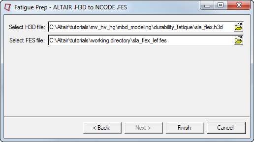
 (Open Document).

 .
.
 (Open Model).
 (Start/Pause Animation) button
to animate the model. Observe the model, which is a combination of rigid
multi-bodies and two flexible lower control arms.
(Start/Pause Animation) button
to animate the model. Observe the model, which is a combination of rigid
multi-bodies and two flexible lower control arms. (Contour).
You can choose different options from the Result Type drop-down menu to view the various results available in the analysis result files.Tip: For a detailed description of writing a fatigue analysis file from here, refer to the Fatigue Manager topic in the HyperView User’s Guide.
(Contour).
You can choose different options from the Result Type drop-down menu to view the various results available in the analysis result files.Tip: For a detailed description of writing a fatigue analysis file from here, refer to the Fatigue Manager topic in the HyperView User’s Guide.