ACU-T: 7010 Shape Optimization using HyperStudy
Prerequisites
Prior to starting this tutorial, you should have already run through the introductory tutorial, ACU-T: 1000 HyperWorks UI Introduction, and have a basic understanding of HyperMesh, AcuSolve, and HyperView. To run this simulation, you will need access to a licensed version of HyperMesh and AcuSolve.
Prior to running through this tutorial, copy HyperMesh_tutorial_inputs.zip from <Altair_installation_directory>\hwcfdsolvers\acusolve\win64\model_files\tutorials\AcuSolve to a local directory. Extract ACU-T7010_HyperStudy.hm from HyperMesh_tutorial_inputs.zip.
Since the HyperMesh database (.hm file) contains meshed geometry, this tutorial does not include steps related to geometry import and mesh generation.
Problem Description
The geometry for this problem consists of a simple pipe channel with perfectly circular cross-section as the base shape. Water enters the Inlet at the rate of 0.0003 kg/s and the outlet is a standard pressure outlet at zero relative pressure. Walls of the channel are no-slip walls.

Figure 1.
Open the HyperMesh Model Database
-
Click the Open Model icon
 located on the standard toolbar.
The Open Model dialog opens.
located on the standard toolbar.
The Open Model dialog opens.
Specify the Boundary Conditions
By default, all components are assigned to the wall boundary condition. In this step, you will change them to the appropriate boundary conditions and assign material properties to the fluid volumes.
-
Click Fluid. In the Entity Editor,
- Change the Type to FLUID.
- Set the Material to Air_HM.
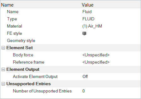
Figure 2. -
Click Inflow. In the Entity Editor,
- Change the Type to INFLOW.
- Change the Inflow type to Mass flux.
- Set the Mass flux value to 0.0003 kg/sec.
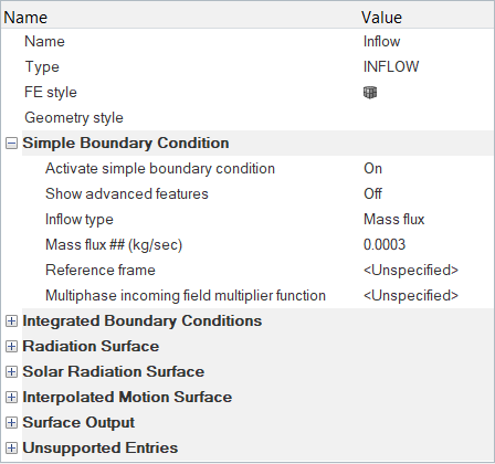
Figure 3. -
Click Outflow. In the Entity Editor, change the Type to
OUTLFOW and leave the remaining options as
default.
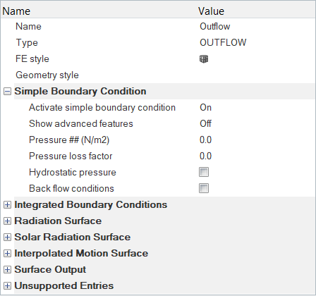
Figure 4. -
Click Wall. In the Entity Editor, verify that the Type is set to WALL.
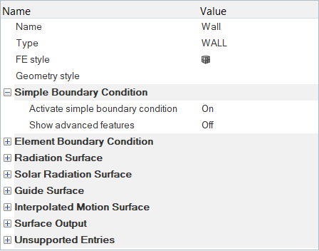
Figure 5.
Set the Optimization Parameters
Generate and Export Morph Shapes
-
Click create.
A new morph volume is created.
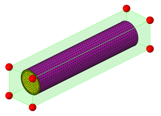
Figure 6. -
Go to the split/combine sub-panel. In the panel area, toggle the option to # of
splits and set it to 3.
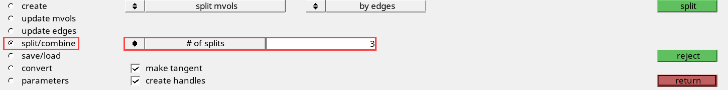
Figure 7. -
In the graphics area, select the edge shown in the figure below.
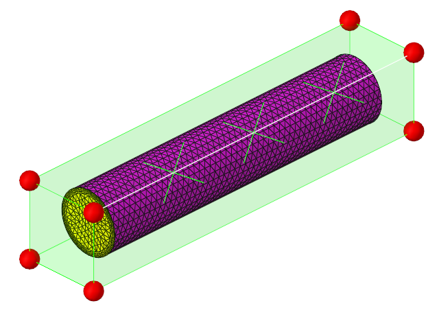
Figure 8. -
In the panel area, click
split.
The morph volume is split into smaller volumes.
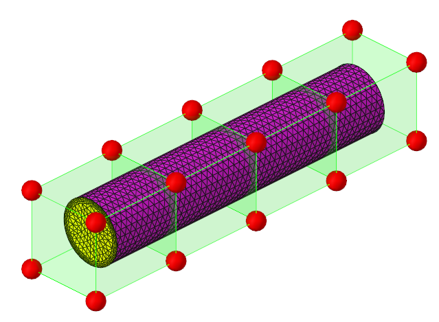
Figure 9. -
In the panel area, go to the update
edges sub-panel. Click the first arrow and select
update ends. Then, click the second arrow and select
by mvols. Finally, click the third arrow and select
the main-secondary option.
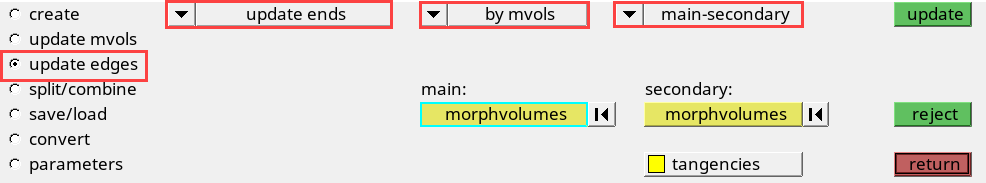
Figure 10. -
Activate the main morphvolmes collector and select the
outer two morph volumes shown in the figure below. Then, activate the
secondary morphvolumes collector and select the inner
two morph volumes.
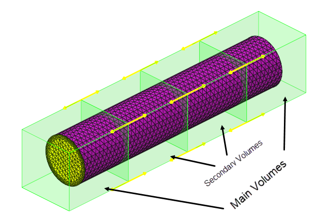
Figure 11. -
After selecting the volumes in the order mentioned, click
update.
The edges in the volume should resemble the figure shown below.
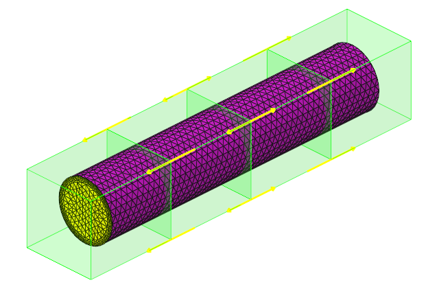
Figure 12. -
Click return to go the HyperMorph panel. Select morph in
the panel area then select the move
handles sub-panel. In this panel,
- Click the second arrow and change it from interactive to translate.
- Below that, click the arrow and select along vector.
- Under that, set the orientation selector to y-axis.
- In the dist= field, enter 0.01.
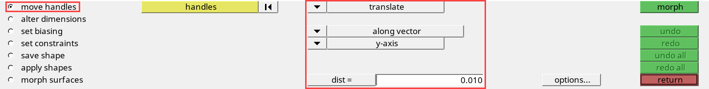
Figure 13. -
Activate the handles collector and select the four
middle handles as shown in the figure below.
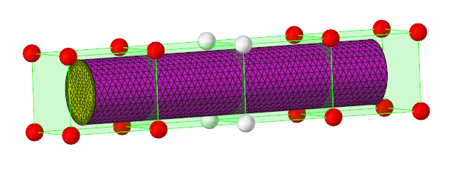
Figure 14. -
In the panel area, click
morph.
The grid is morphed.
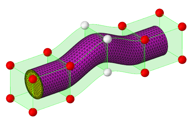
Figure 15.
Define the Design Variable
-
Click create to create a design variable named
'bend'.
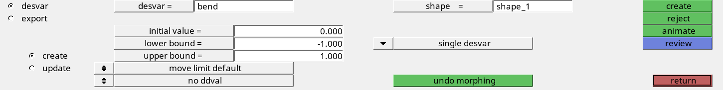
Figure 16.
Launch the DOE Study Using HyperStudy
Start the Nominal Run
-
Click
 on the CFD toolbar.
The HyperStudy Job Launcher dialog.
on the CFD toolbar.
The HyperStudy Job Launcher dialog. -
Click Launch.
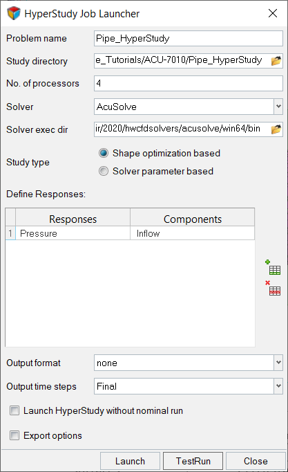
Figure 17.
In the HyperStudy window, check step by step by clicking on each setup from the Explorer menu to ensure that everything was properly defined.
Run the DOE Study
-
In the Explorer window, right-click on Study 1 and
select Add.
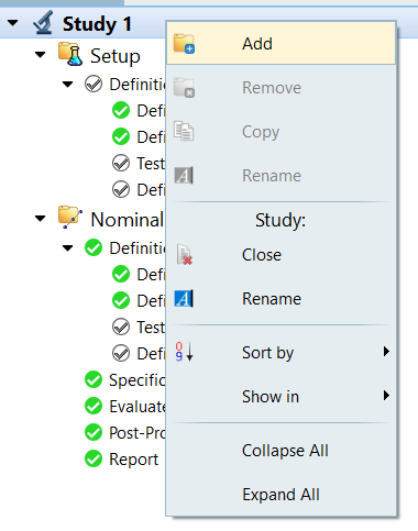
Figure 18. -
In the Work Area, set the Mode to Full Factorial by
expanding the Show more… option.
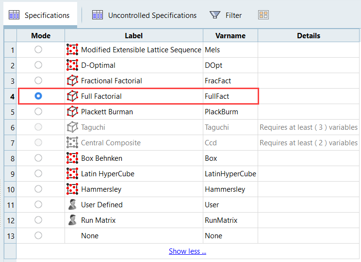
Figure 19. -
Click the Levels tab, set the number of levels to
5, then click Apply.
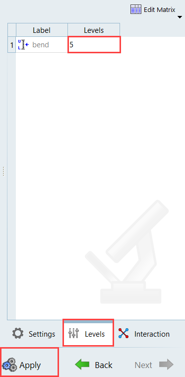
Figure 20. -
In the Explorer, click Evaluate under DOE 1.
The table used to run the study appears, showing all of the runs (1 - 5) to be executed.
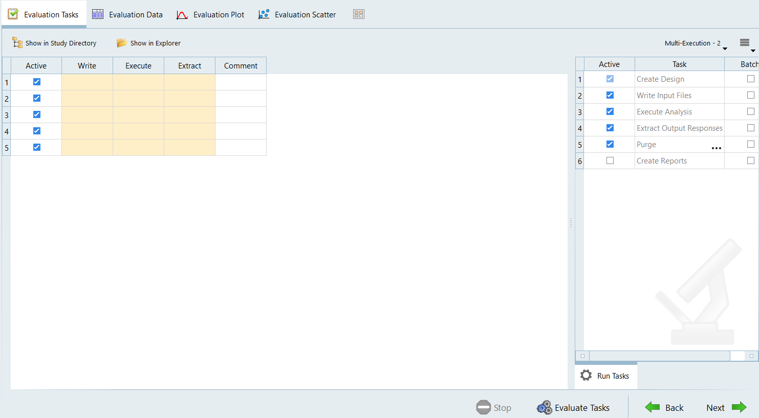
Figure 21. -
Once all the runs are complete, click the Evaluation
Data tab.
The table displays the list of values used for the design variable and also the corresponding value of the response variable (inflow pressure).
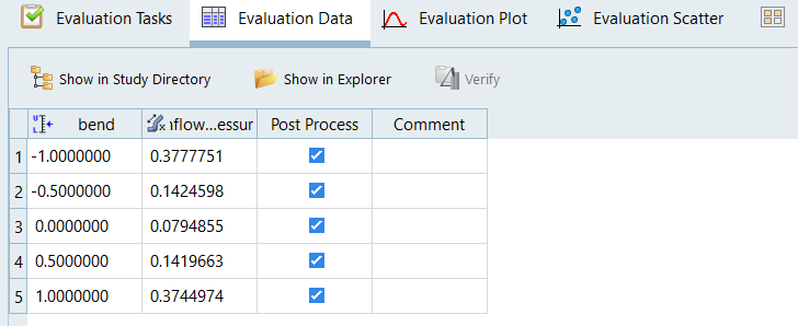
Figure 22. -
Plot the values of the response variable (inflow pressure) by selecting it in
the Channel selector.
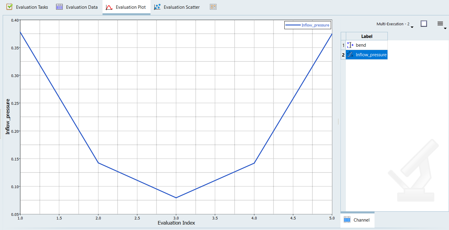
Figure 23.You can also plot the list of design variables by switching the label to bend.
Post-Process the Results with HyperView
Switch to the HyperView Interface and Load the AcuSolve Model and Results
-
In the HyperMesh Desktop window, click the
ClientSelector drop-down in the bottom-left corner of
the graphics window.
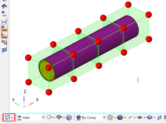
Figure 24. -
In the Load model and results panel, click
 next
to Load model.
next
to Load model.
Create a Pressure Contour on a Cut Plane
-
Click
 on the Results toolbar to open the Contour panel.
-
Click the Section cut icon
 on the HV-Display toolbar.
-
Click Gridline. In the Gridline
Options dialog, deactivate the Show check
box under Grid line then click OK.
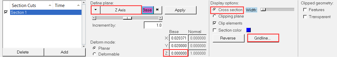
Figure 25. -
Orient the display to the xy-plane by clicking
 on the Standard Views toolbar.
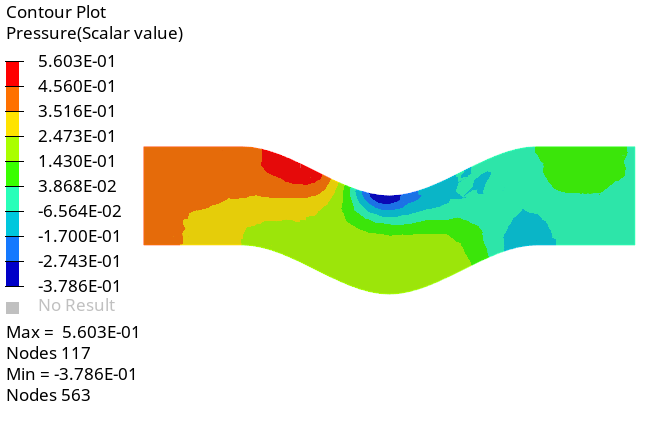
Figure 26. Run 1 -
Repeat the above steps to create a contour plot of pressure for each individual
run using the respective log files.
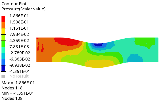
Figure 27. Run 2
Figure 28. Run 3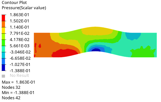
Figure 29. Run 4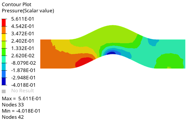
Figure 30. Run 5
Summary
This tutorial introduced you to running a DOE study using Altair products, namely HyperMesh, AcuSolve, HyperStudy and HyperView. You started by importing a HyperMesh database and then set up the simulation parameters for AcuSolve and created a morph shape using HyperMorph. Next, you set up the design variable and linked the morph shape to it. Then, you proceeded to set up the DOE study. Once the results were obtained, you processed the results using HyperView.