ACU-T: 7001 Shape Optimization using HyperMorph
Prerequisites
Prior to starting this tutorial, you should have already run through the introductory tutorial, ACU-T: 1000 HyperWorks UI Introduction, and have a basic understanding of HyperMesh, AcuSolve, and HyperView. To run this simulation, you will need access to a licensed version of HyperMesh and AcuSolve.
Prior to running through this tutorial, copy HyperMesh_tutorial_inputs.zip from <Altair_installation_directory>\hwcfdsolvers\acusolve\win64\model_files\tutorials\AcuSolve to a local directory. Extract ACU-T7001_ShapeOptimization.hm from HyperMesh_tutorial_inputs.zip.
Since the HyperMesh database (.hm file) contains meshed geometry, this tutorial does not include steps related to geometry import and mesh generation.
Problem Description
Optimization, in simple terms, is the process of selecting a best input from a set of available alternatives. AcuSolve offers you two options to setting up an optimization study: design optimization and parametric studies. Design optimization enables you to optimize an objective function subject to certain constraints and satisfaction of flow equations. The design optimization may be considered as a sequence of cases, where each case first runs the optimizer and updates the design variables and then solves the flow equations for a number of time steps until convergence. Sample data is gathered at the end of each time step.
The optimizer solution consists of:
- Constructing the response surface from the set of samples.
- Running the optimizer on the response surface.
- Updating the design variables.
The geometry for this problem consists of a simple pipe channel with perfectly circular cross-section as the base shape. Water enters the Inlet at the rate of 0.0003 kg/s and the outlet is a standard pressure outlet at zero relative pressure. Walls of the channel are no-slip walls.

Figure 1.
Open the HyperMesh Model Database
-
Click the Open Model icon
 located on the standard toolbar.
The Open Model dialog opens.
located on the standard toolbar.
The Open Model dialog opens.
Set the Global Simulation Parameters
Set the Analysis Parameters
-
Set the Mesh type to Fully Specified.
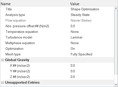
Figure 2.
Specify the Solver Settings
-
Check that the Flow and Design Optimization flags are set to On.
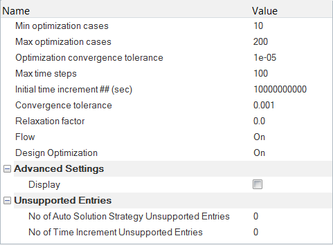
Figure 3.
Set the Nodal Output Frequency
Create Mesh Motion and Set the Boundary Conditions and Material Model Parameters
Create Mesh Motion
An optimization study can be performed in AcuSolve using either volume morph shapes or surface morph shapes. If volume morph shapes are used for simulation, you do not need to define mesh motion, as the volume nodes will move using the input from morph shapes. If surface morph shapes are used for simulation, interpolated mesh motion is needed to define the motion of volume nodes in the model. For this tutorial, surface morph shapes with interpolated mesh motion is used.
-
Set the Type to Interpolated_Motion and the Number of
Interpolated surfs to 3.
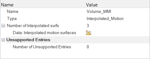
Figure 4. -
Click the data entry icon
 .
The Number of Interpolates surfs dialog opens.
.
The Number of Interpolates surfs dialog opens. -
Select Wall, Inflow, and
Outflow.
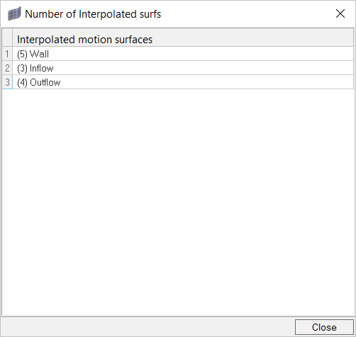
Figure 5.
Specify the Boundary Conditions and Material Models Parameters
-
Click Inflow. In the Entity Editor,
- Change the Type to INFLOW.
- Set the Inflow type to Mass flux.
- Set the Mass flux to 0.0003 kg/sec
- Under the Interpolated Motion Surface section, turn on Display and Activate the interpolated motion surface.
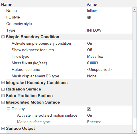
Figure 6. -
Click Outflow. In the Entity Editor,
- Change the Type to OUTFLOW.
- Under the Interpolated Motion Surface section, turn on Display and Activate the interpolated motion surface.
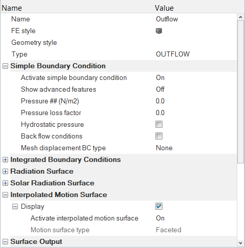
Figure 7. -
Click Wall. In the Entity Editor,
- Verify that the Type ia set to Wall.
- Under the Interpolated Motion Surface section, turn on Display and Activate the interpolated motion surface.
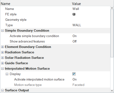
Figure 8. -
Click Fluid. In the Entity Editor,
- Change the Type to FLUID.
- Select Water_HM as the Material.
- Set the Mesh motion to Volume_MMI.
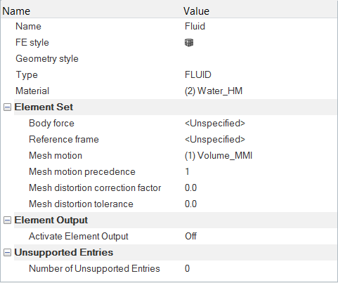
Figure 9.
Set Up Optimization Parameters
Generate and Export Morph Shapes
HyperMorph is used to parameterize the shape of the design. You will create morph shapes by moving the surface nodes. The volume nodes will be taken care of using the interpolated mesh motion feature of HyperMesh.
-
In the morphing sub-panel, change mvols:active to mvols:skin
only.
By changing this option to “skin only”, you only morph the surfaces and surface morph shapes are generated. If “mvols” is left to default, volume morph shapes are generated where all the nodes in the model are deformed (not just surfaces) during the morphing process.
Important: Do not click the solve button.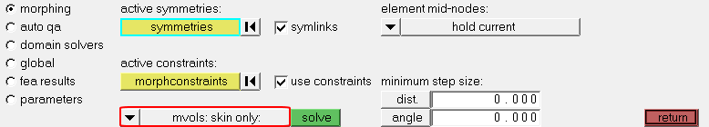
Figure 10. -
Click create.
A new morph volume is created.
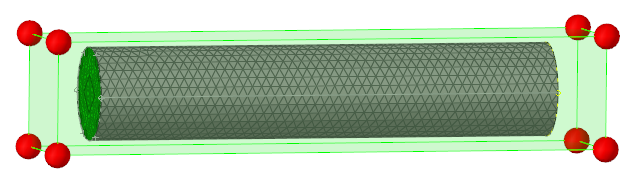
Figure 11. -
Select the move handles sub-panel if it's not already
selected. In the sub-panel, click the second arrow and select
scale. Leave the x scale at 1.0 and set the y scale
and z scale to 1.5.
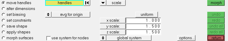
Figure 12. -
In the modeling window, select the four edge handles at
the pipe outflow, highlighted in grey in the figure below.
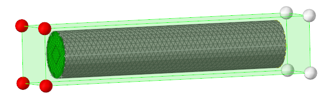
Figure 13. -
Click morph.
The grid is morphed.
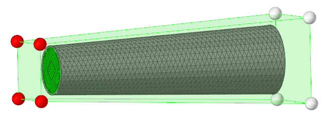
Figure 14. -
Select the save shape sub-panel. In this panel,
- Set the name field to outflow_expand.
- In the second row, set the selector to as node perturbations.
- Check that the coordinate system is set to global and click save.
- Select No when asked to “Save perturbations for nodes at global and morph volume handles?”
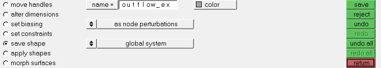
Figure 15.Note: When you click save, a new entity folder, Shapes, will be created in the Model Browser. The shape outflow_expand will be created inside this folder in the Model Browser. You can turn off the display of the shape nodal perturbations by right-clicking on outflow_expand and selecting Hide. To show the shape again, right-click on outflow_expand and select Show. It is recommended to hide the shape display at this point before proceeding to next steps. -
Click morph.
The grid is morphed.
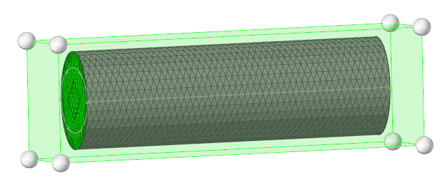
Figure 16. -
In the second row, set the split type to No. of splits (# of
splits) and enter 3 for the number of
splits.
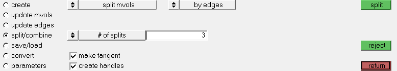
Figure 17. -
In the modeling window, select the edge of the morph
volume marked by green crosses in the figure below.
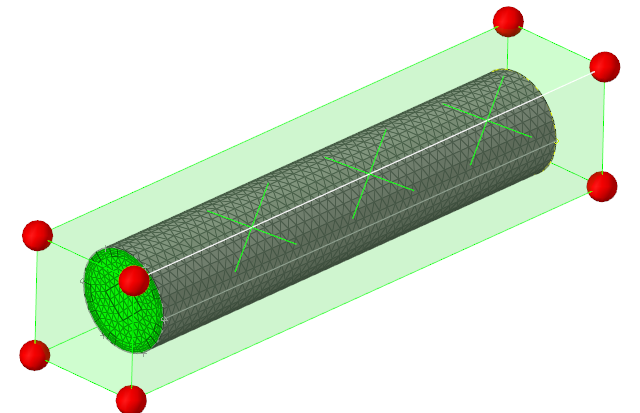
Figure 18. -
Click update edges to open the corresponding sub-panel.
Click the first arrow and select update ends. Then, click
the second arrow and select mvols. Finally, click the
third arrow and select main-secondary.
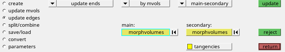
Figure 19.Note: This option allows you to link any two edges together with a main-secondary relationship between two morph volumes. In this kind of relationship, the secondary edge is forced to follow the curvature of the main edge at the joining end of the two edges. -
Activate the main morphvolmes collector and select the
outer two morph volumes shown in the figure below. Then, activate the
secondary morphvolumes collector and select the inner
two morph volumes. After selecting the volumes in the order mentioned, click
update.
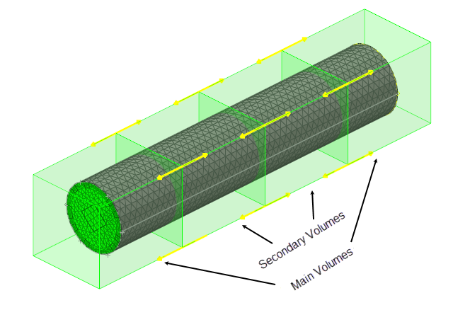
Figure 20.The edges in the volume should resemble the figure shown below.
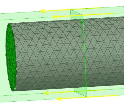
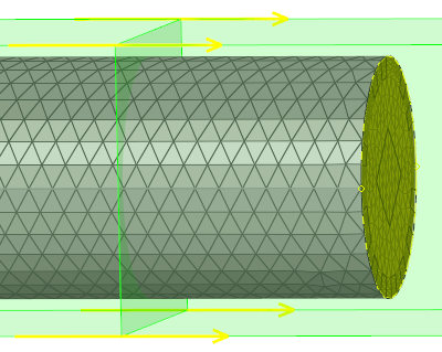
Figure 21.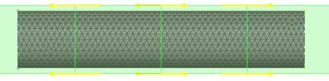
-
Activate the handles collector by clicking on it then
select the four middle handles in the modeling window.
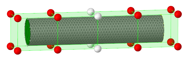
Figure 22. -
Click morph.
The grid is morphed.
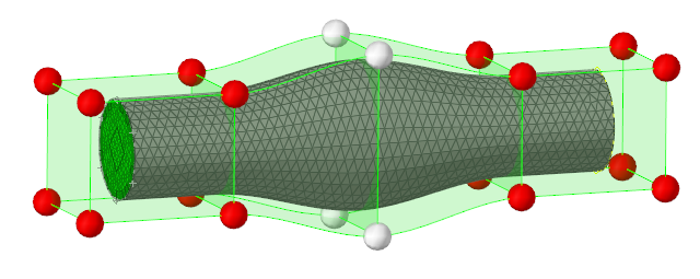
Figure 23.
Define the Design Variable
- Right-click on 10.Optimization in the Solver Browser and select from the context menu.
- Rename the variable to outflow_expand and press Enter.
- In the Entity Editor, set the Initial Value to 0.7.
- Set the Lower Bound to 0.2.
- Set the Upper Bound to 1.5.
- Set the Max Update Factor to 0.02.
- Follow the above steps to create two new design variables, length_z and center_y. Use identical parameters as above to define these two new design variables.
Define the Response Variable
-
Change the Output variable to Pressure.
This response variable will extract the surface integrated value of the pressure variable from the inflow surface.
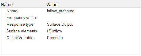
Figure 24.
Define the Objective
- Right-click on Optimization in the Solver Browser and select from the context menu.
- Rename the objective to maximize_inflow_pressure and press Enter
- In the Entity Editor, set the Objective Type is set to Maximize.
- Select inflow_pressure as the Response variable.
Set Up the Nodal Shapes
-
Similarly, select length_z as the shape and design
variable for row 2 and center_y as the shape and design
variable for row 3.
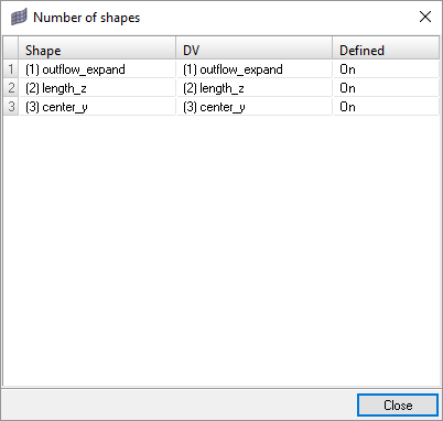
Figure 25.
Set Up Optimization Controls
- In the Entity Editor, expand .
- In the Entity Editor, select maximize_inflow_pressure as the Objective.
- Verify that the Optimizer convergence tolerance is set to 1e-4.
- Save the model.
Compute the Solution
In this step, you will launch AcuSolve directly from HyperMesh and compute the solution.
Run AcuSolve
-
Click
 on the ACU toolbar.
The Solver job Launcher dialog opens.
on the ACU toolbar.
The Solver job Launcher dialog opens. -
Leave the remaining options as
default and click Launch to start the solution
process.
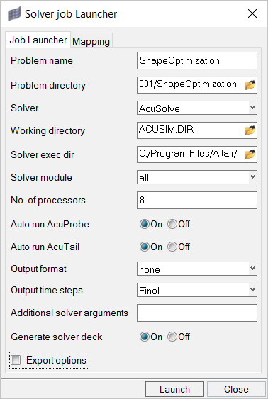
Figure 26.
Monitor the Solution with AcuProbe
AcuProbe can be used to monitor various variables over solution time. An AcuProbe window will be launched by the Solver Job Launcher if the Auto run AcuProbe flag is set to On.
-
Right-click on pressure and select
Plot.
Note: You might need to click
 on the toolbar in order to
properly display the plot.
on the toolbar in order to
properly display the plot. -
Select to change the x-axis from Time Step to Case ID.
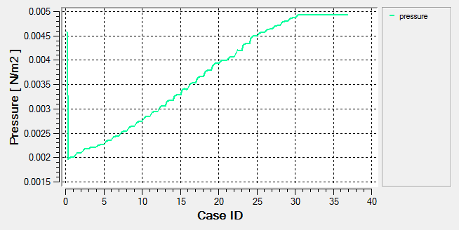
Figure 27.
AcuGetDv and AcuGetRsp
AcuSolve provides two post-processing utilities specific to optimization problems, AcuGetDv and AcuGetRsp. AcuGetDv provides the values of the design variables for all the cases included in the solution. AcuGetRsp provides the values of the response variables for all the cases included in the solution.
-
Enter the following command at the prompt:
acuGetDv
AcuSolve will print the values of design variables for each case.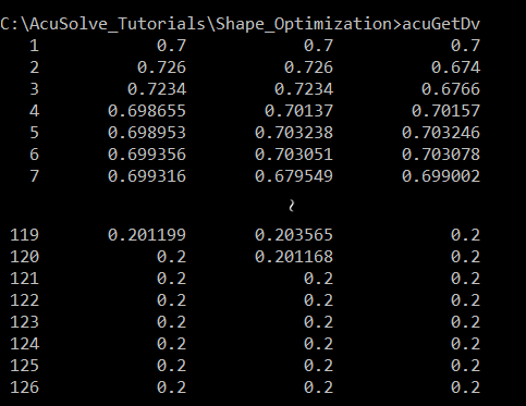
Figure 28. -
To print the values of response variables, use the command:
acuGetRsp
Note: The order of columns in which the design variables and the response variables are printed by these commands is the order in which they appear in the INP file.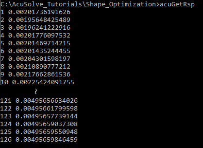
Figure 29.
Post-Process the Results with HyperView
Open HyperView and Load the Model and Results
-
In the Load model and results panel, click
 next
to Load model.
next
to Load model.
Create the Pressure Variation Animation
-
Click
 on the Results toolbar to open the Contour panel.
-
In the panel area, under the Display tab, turn off
the Discrete color option.
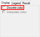
Figure 30. -
On the Animation toolbar, click the Animation Controls icon
 .
.
-
Click the Start/Pause Animation icon
 to play the animation in the graphics area.
Save the Animation
-
On the ImageCapture toolbar, make sure that the Save Image to File option is
On.
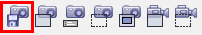
-
Click the Capture Graphics Area Video icon
 .
The Save Graphics Area Video As dialog opens.
.
The Save Graphics Area Video As dialog opens.
Summary
In this tutorial, you learned how to set up and solve a shape optimization problem with AcuSolve using HyperMorph. You started by importing the model database and then created mesh morphs. Then, you defined the design variables, the response variables, and set up the objectives of the problem using the response variables. Once the solution was computed using AcuSolve, you used the AcuSolve Command Prompt to get the design variables and response variables used for the optimization cases. Finally, you used HyperView to visualize how the shape of the pipe changed with the optimization steps.