Fatigue Process
Create or open a fatigue analysis setup process.
The fatigue process template is a workflow-based process manager framework. It is supported on the HyperWorks Desktop environment. It allows you to set up a quick OptiStruct solver deck for fatigue simulation with minimum intervention. It also allows you to submit the OS job on the local workstation and supports post processing of fatigue results such as life & damage within the same environment.
- Importing the model
- Creating the fatigue subcase
- Defining fatigue analysis parameters
- Defining fatigue elements and SN/EN properties
- Defining the load-time history and the loading sequence
- Submitting the job
- Viewing the results summary and launching HyperView for post-processing
Create New Session
In this step you will create a new fatigue process session.
-
From the menu bar, click .
The Create New Session dialog opens.
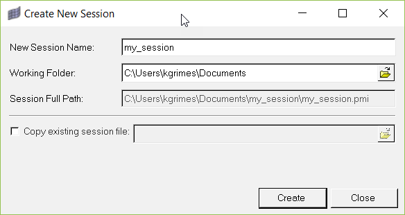
Figure 1. -
Click Create.
The panel area displays similar to the following image.
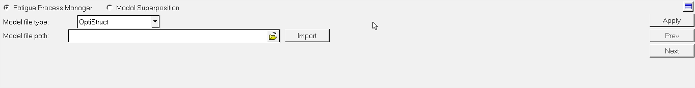
Figure 2. -
Click Apply to move on to the
next step in the process.
The Process Manager browser will move to the Fatigue Subcase step and the panel displays similar to the following image.
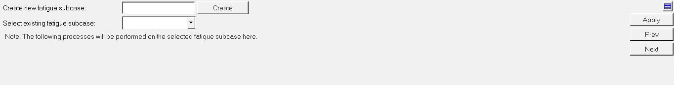
Figure 3.
Load Existing Session
As an alternative to creating a new fatigue process session, you can load an existing session if you have one already saved.
-
Click Apply to move on to the
next step in the process.
The Process Manager browser moves to the Fatigue Subcase step and the panel displays similar to the following image.
Figure 4.
Create Fatigue Subcase
In this step you are prompted to create a fatigue subcase. A fatigue subcase is used to link fatigue loads, events, and analysis parameters together for a fatigue simulation. This subcase will remain active so that other fatigue cards created in subsequent steps will be tied to this active fatigue subcase.
-
Click Apply to move on to the
next step in the process.
The Process Manager browser will move to the Analysis Parameters step and the panel displays similar to the following image.
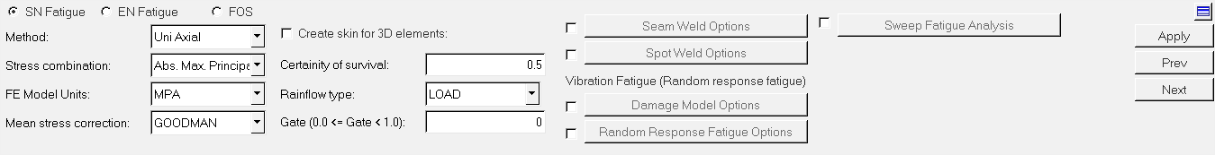
Figure 5.
Define Analysis Parameters
In this step you will define all parameters required for a fatigue analysis. Parameters include fatigue analysis type, stress combination methods, stress tensor units, and so forth. The parameters displayed in the panel area will change depending on your selection of fatigue type.
SN Fatigue Uniaxial
In this step you will set parameters for the SN Fatigue Uniaxial option.
-
Select the SN Fatigue option at the top of the Fatigue
Process panel and then select Uni Axial as the Method.
The panel displays similar to the following image.
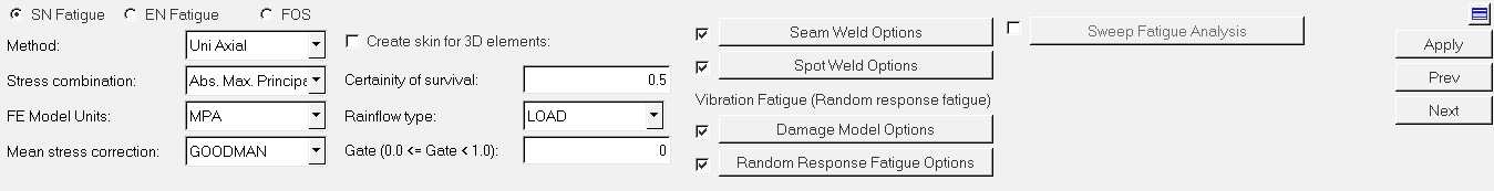
Figure 6.Some of the parameters require selection from drop-down menus, while others require you to place a checkmark in the appropriate checkbox and then click the respective button. Make your selections according to the following table.Parameter definitions can be found in the OptiStruct Reference Guide.Parameter Name Values Method Uni Axial or Multi Axial Stress Combination Max. Principal, Min Principal, Abs. Max. Principal, Von Mises, Signed Von Mises, Tresca, Signed Tresca, Signed Max. Shear, XYZ Normal, XY Shear, YZ Shear, or ZX Shear FE Model Units MPA, PA, PSI, or KSI Mean Stress Correction None, Goodman, Gerber, Gerber2, Soderbe, FKM, or FKM2 Create Skin for 3D Elements Checked or Unchecked Certainty of Survival <value> Rainflow Type Load or Stress Gate (0.0 <= Gate < 1.0) <value> Seam Weld Options Checked or Unchecked, then click button - Method: Volvo
- Mean Stress Correction: None or FKM
- Certainty of Survival: <value>
- Thickness Correction: Yes or No
Spot Weld Options Checked or Unchecked, then click button - Method: Rupp
- Mean Stress Correction: None or FKM
- Certainty of Survival: <value>
- Thickness Correction: Yes or No
- No. of Angles on Sheet: <value>
Damage Model Options Checked or Unchecked, then click button - DM1 through DM4: DIRLIK, LALANNE, NARROW, or THREE
Random Response Fatigue Options Checked or Unchecked, then click button - Upper Limit of Stress Range (FACSREND): <value>
- Upper Limit of Stress Range (SREND): <value>
- Width of Stress Ranges (NBIN): <value>
- Width of Stress Ranges (DS): <value>
- Static Subcase (STSUBID): select a subcase
Sweep Fatigue Analysis Checked or Unchecked, then click button - NF_OPTION: checked or unchecked
- NF: NFREQ
- DF: <value>
- Static Subcase (STSUBID): select a subcase
-
Click Apply to move on to the next step in the
process.
The Process Manager browser will move to the Elements and Materials step and the panel displays similar to the following image.
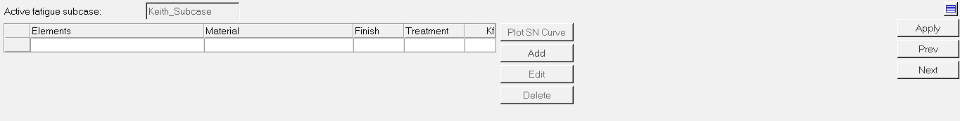
Figure 7.
SN Fatigue Multiaxial
In this step you will set parameters for the SN Fatigue Multiaxial option.
-
Select the SN Fatigue option at the top of the
Fatigue Process panel and then select
Multi Axial as the Method. The
panel displays similar to the following image.
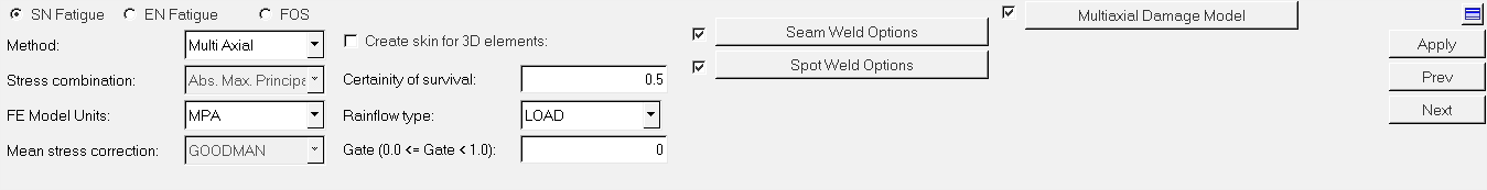
Figure 8.Some of the parameters require selection from drop-down menus, while others require you to place a checkmark in the appropriate checkbox and then click the respective button. Make your selections according to the following table.Parameter definitions can be found in the OptiStruct Reference Guide.Parameter Name Values Method Uni Axial or Multi Axial Stress Combination Set to Max. Abs. Principal by default FE Model Units MPA, PA, PSI, or KSI Mean Stress Correction Set to Goodman by default Create Skin for 3D Elements Checked or Unchecked Certainty of Survival <value> Rainflow Type Load or Stress Gate (0.0 <= Gate < 1.0) <value> Seam Weld Options Checked or Unchecked, then click button - Method: Volvo
- Mean Stress Correction: None or FKM
- Certainty of Survival: <value>
- Thickness Correction: Yes or No
Spot Weld Options Checked or Unchecked, then click button - Method: Rupp
- Mean Stress Correction: None or FKM
- Certainty of Survival: <value>
- Thickness Correction: Yes or No
- No. of Angles on Sheet: <value>
Multiaxial Damage Model Checked or Unchecked, then click button - DM1 through DM3: GOODMAN (Tension Damage), FKM (Tension Damage), or FINDLEY (Shear Damage)
-
Click Apply to move on to the
next step in the process.
The Process Manager browser will move to the Elements and Materials step and the panel displays similar to the following image.
Figure 9.
EN Fatigue Uniaxial
In this step you will set parameters for the EN Fatigue Uniaxial option.
-
Select the EN Fatigue option at the top of the
Fatigue Process panel and then select Uni
Axial as the Method. The panel displays
similar to the following image.
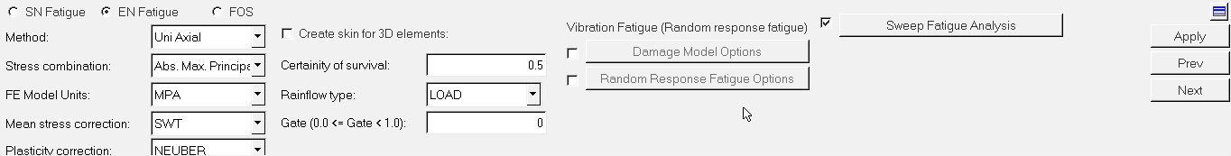
Figure 10.Some of the parameters require selection from drop-down menus, while others require you to place a checkmark in the appropriate checkbox and then click the respective button. Make your selections according to the following table.Parameter definitions can be found in the OptiStruct Reference Guide.Parameter Name Values Method Uni Axial or Multi Axial Stress Combination Set to Max. Abs. Principal by default FE Model Units MPA, PA, PSI, or KSI Mean Stress Correction NONE, MORROW, MORROW2, or SWT Plasticity Correction NEUBER or NONE Create Skin for 3D Elements Checked or Unchecked Certainty of Survival <value> Rainflow Type Load or Stress Gate (0.0 <= Gate < 1.0) <value> Damage Model Options Checked or Unchecked, then click button - DM1 through DM4: DIRLIK, LALANNE, NARROW, or THREE
Random Response Fatigue Options Checked or Unchecked, then click button - Upper Limit of Stress Range (FACSREND): <value>
- Upper Limit of Stress Range (SREND): <value>
- Width of Stress Ranges (NBIN): <value>
- Width of Stress Ranges (DS): <value>
- Static Subcase (STSUBID): select a subcase
Sweep Fatigue Analysis Checked or Unchecked, then click button - NF_OPTION: checked or unchecked
- NF: NFREQ
- DF: <value>
- Static Subcase (STSUBID): select a subcase
-
Click Apply to move on to the
next step in the process.
The Process Manager browser will move to the Elements and Materials step and the panel displays similar to the following image.
Figure 11.
EN Fatigue Multiaxial
In this step you will set parameters for the EN Fatigue Multiaxial option.
-
Select the EN Fatigue option at the top of the Fatigue
Process panel and then select Multi Axial as the Method.
The panel displays similar to the following image.
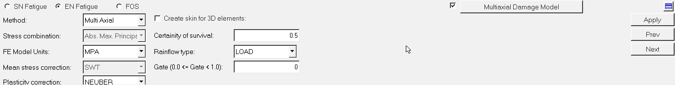
Figure 12.Some of the parameters require selection from drop-down menus, while others require you to place a checkmark in the appropriate checkbox and then click the respective button. Make your selections according to the following table.Parameter definitions can be found in the OptiStruct Reference Guide.Parameter Name Values Method Uni Axial or Multi Axial Stress Combination Set to Max. Abs. Principal by default FE Model Units MPA, PA, PSI, or KSI Mean Stress Correction Set to SWT by default Plasticity Correction NEUBER or NONE Create Skin for 3D Elements Checked or Unchecked Certainty of Survival <value> Rainflow Type Load or Stress Gate (0.0 <= Gate < 1.0) <value> Multiaxial Damage Model Checked or Unchecked, then click button - DM1 through DM4: SWT (Tension Damage), FS (Shear Damage), BM (Shear Damage), or MORROW (Tension Damage)
-
Click Apply to move on to the
next step in the process.
The Process Manager browser moves to the Elements and Materials step and the panel displays similar to the following image.
Figure 13.
Factor of Safety (FOS)
In this step you will set parameters for the Factor of Safety (FOS) option.
-
Select the FOS option at the top of the Fatigue Process
panel. The panel displays similar to the following image.
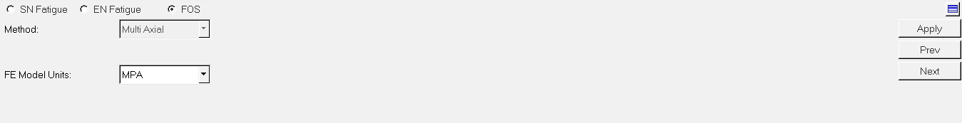
Figure 14.Some of the parameters require selection from drop-down menus, while others require you to place a checkmark in the appropriate checkbox and then click the respective button. Make your selections according to the following table.Parameter Name Values Method Set to Multi Axial by default FE Model Units MPA, PA, PSI, or KSI -
Click Apply to move on to the
next step in the process.
The Process Manager browser will move to the Elements and Materials step and the panel displays similar to the following image.
Figure 15.
Define Elements and Materials
In this step you will identify and define elements and materials to use for fatigue calculation. You can also add spot weld and seam weld material properties to use during fatigue simulation.
SN Material Data
In this step you will define SN materials. This information in this section is useful if you selected SN Fatigue in the previous Analysis Parameters step.
-
In the Elements and Materials panel, click Add.
The Material Data dialog displays.
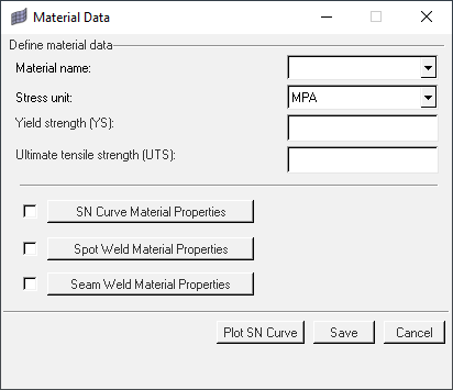
Figure 16. -
Click Plot SN Curve.
Depending on the values you entered into the dialog box, you will see a plot curve similar to the following image.
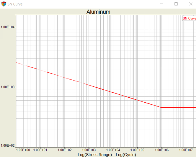
Figure 17. -
Click Add Property. The Property
Data dialog displays.
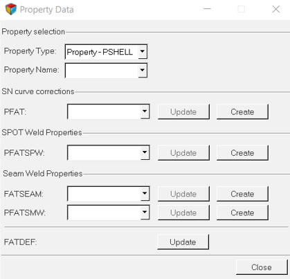 Figure 18.
 -
Click Apply to move on to the next step in the
process.
The Process Manager browser moves on to the Load-Time History step and the panel displays the following image.
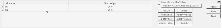 Figure 19.
EN Material Data
In this step you will define EN materials. This information in this section is useful if you selected EN Fatigue in the previous Analysis Parameters step.
-
In the Elements and Materials panel, click Add Material.
The Material Data dialog displays.
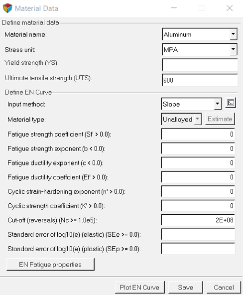
Figure 20. -
Click Plot EN Curve.
Depending on the values you entered into the dialog box, you will see a plot curve similar to the following image.
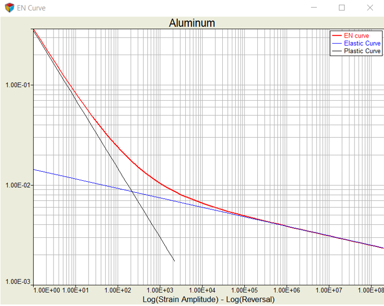
Figure 21. -
Click Add Property.
The Property Data dialog displays.
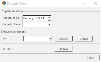
Figure 22. -
Click Apply to move on to the next step in the
process.
The Process Manager browser moves to the Load-Time History step and the panel displays similar to the following image.
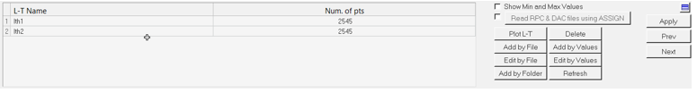 Figure 23.
Loading Information
In this section you will learn how to select and import load-time history data from various sources, such as .csv, DAC and RPC/RSP, to create fatigue cards. After the import process, you can define the sequence of loads to be applied during simulation.
Define Load-Time History
In this step you will import load-time history files.
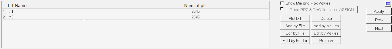
Figure 24.
-
When you are ready to plot the load-time history, select the appropriate row in
the table and click Plot L-T.
You will see a Load-Time History dialog similar to the following image.
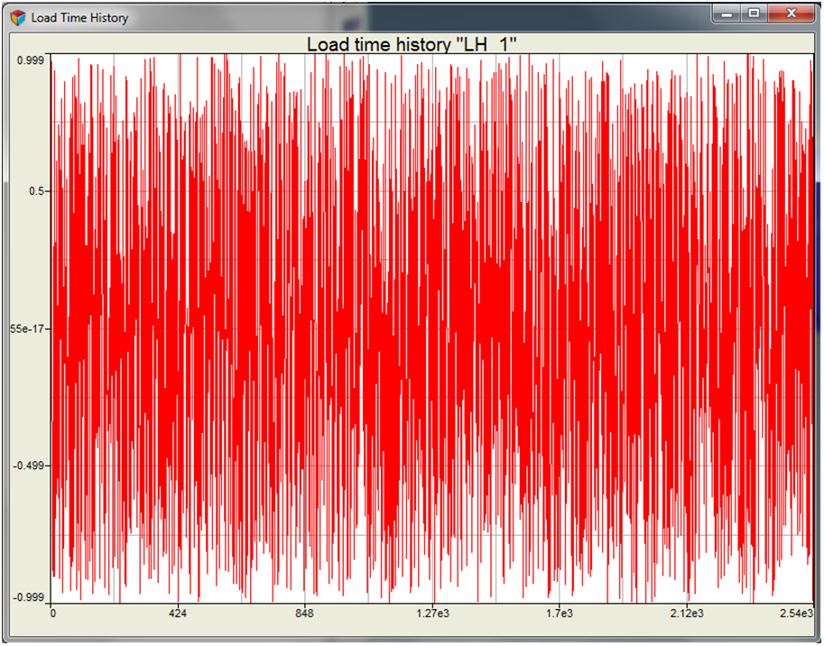
Figure 25. -
Click Apply to move on to the
next step in the fatigue process sequence.
The Process Manager browser will move to the Loading Sequence step and the panel displays similar to the following image.
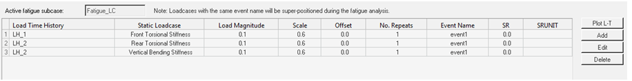
Figure 26.
Define Loading Sequence
In this step you will define the loading sequence.
Figure 27.
-
If you are ready to plot the load-time history based on your existing table,
select a row in the table and click Plot L-T.
You will see a Load-Time History dialog similar to the following image.
Figure 28. -
To add a new row of information to the table:
-
Click Add.
The Load Mapping dialog displays.
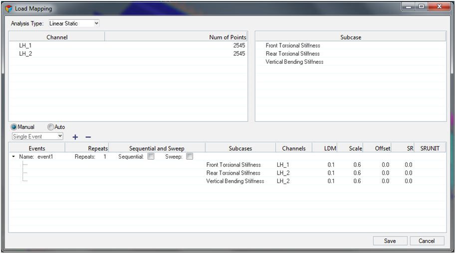
Figure 29.
-
Click Add.
-
Click Apply to move on to the
next step in the fatigue process sequence.
The Process Manager browser moves to the Submit Analysis step and the panel displays similar to the following image.
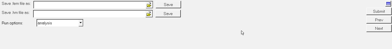
Figure 30.
Submit Analysis
In this step you will learn how to export a solver deck with the appropriate fatigue cards. This process will verify the integrity of the solver card.
-
Click Next to move on to the final step of the fatigue
process.
The panel will switch to the Post Processing panel.

Figure 31.
Post-Processing
In this step you will view post-processing results in HyperView. Doing so allows you to apply contour of fatigue results such as damage or life.
-
Click Apply.
The graphics area updates similar to the following image.
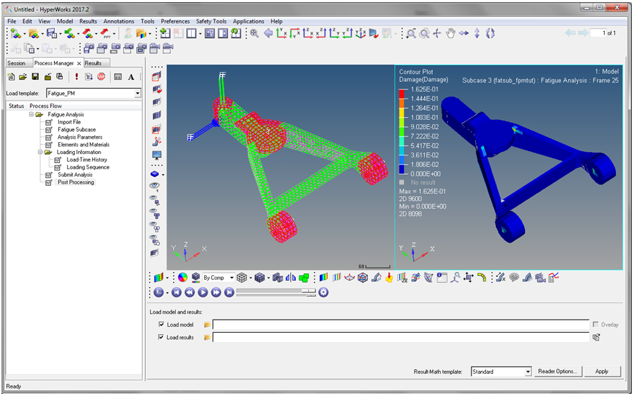
Figure 32.