Hilly Terrain
Calculate propagation in rural/suburban scenario for hilly terrain.
Model Type
The geometry is described by topography (elevation) as well as clutter, see Figure 1. The Database tree enables you to change between topography (terrain elevation at every pixel) and clutter view.
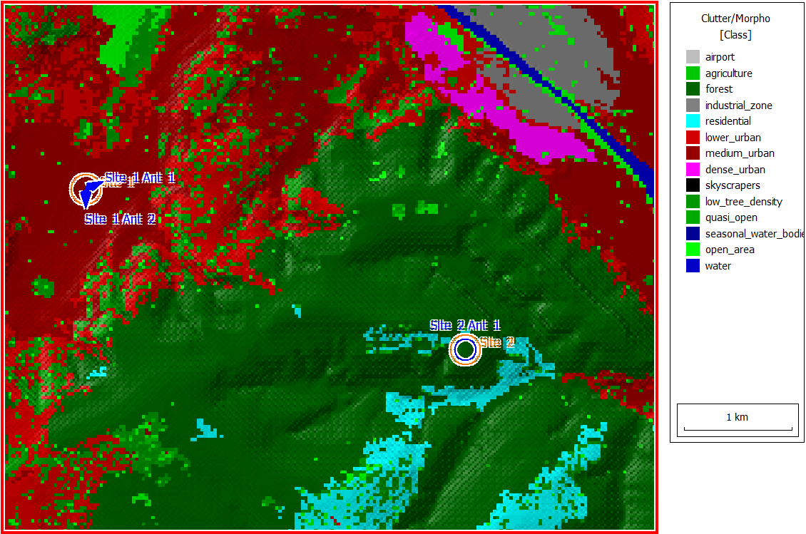
Figure 1. Clutter (land usage).
Sites and Antennas
There are two antenna sites in this scenario. Site 1 has two directional antennas at a height of 25 m, and Site 2 has an omnidirectional antenna at a height of 50 m.
Computational Method
Results
Results are computed for each transmitter at a prediction plane of 1.5 m.
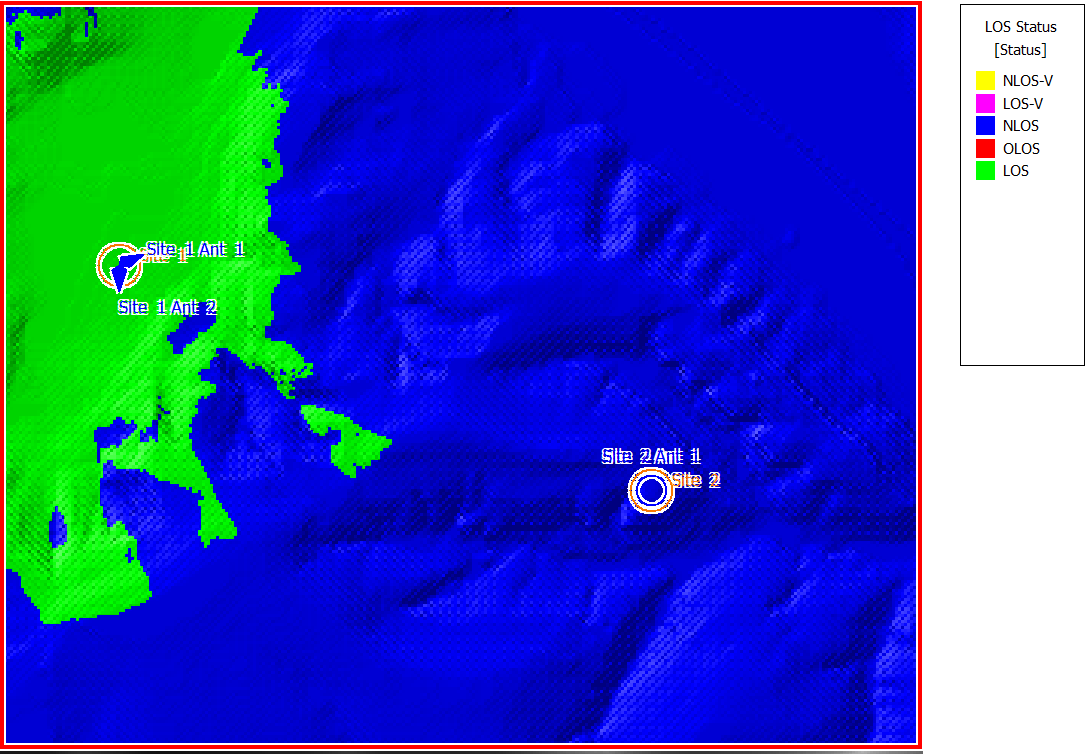
Figure 2. Line-of-sight results for Site-1.
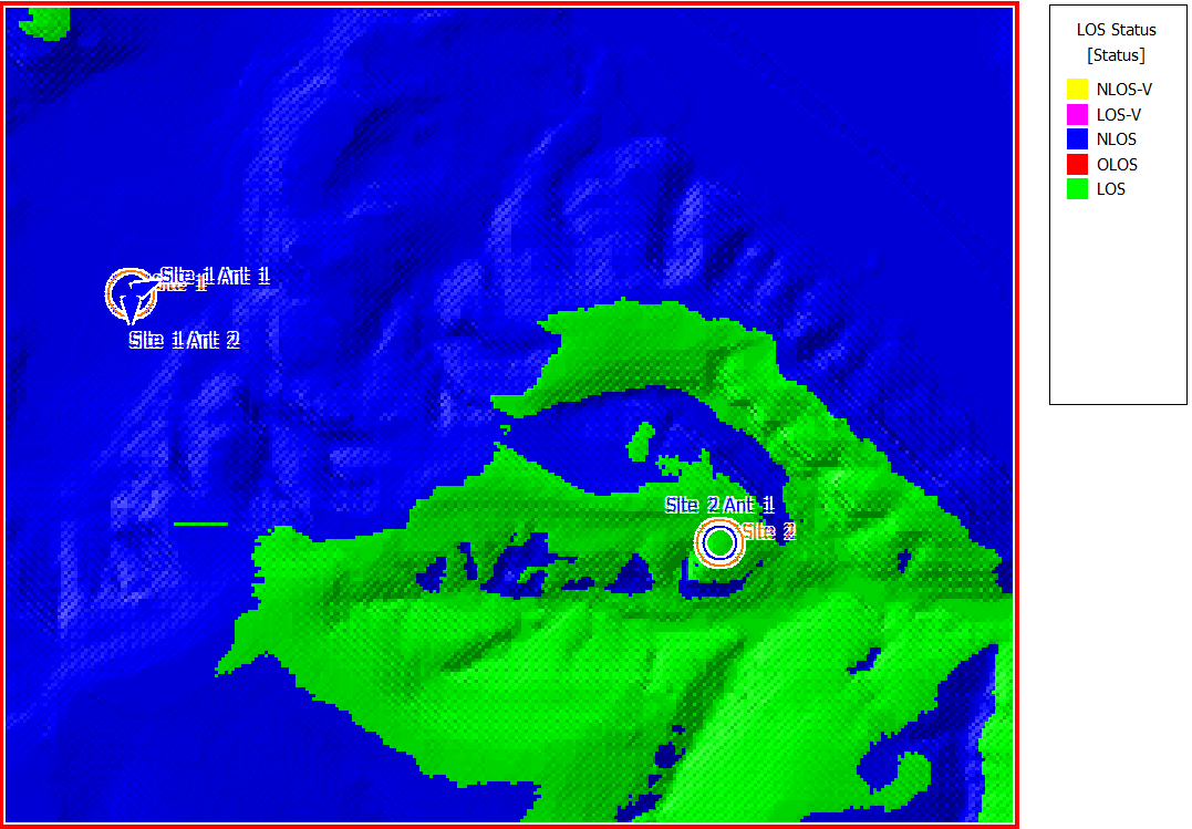
Figure 3. Line-of-sight results for Site-1.
Results for received power are shown in Figure 4. Note the low power levels in non-line-of-sight areas. The Hata-Okumura model on its own would over-estimate the received power in such areas, while the addition of knife-edge diffraction produces more realistic results.
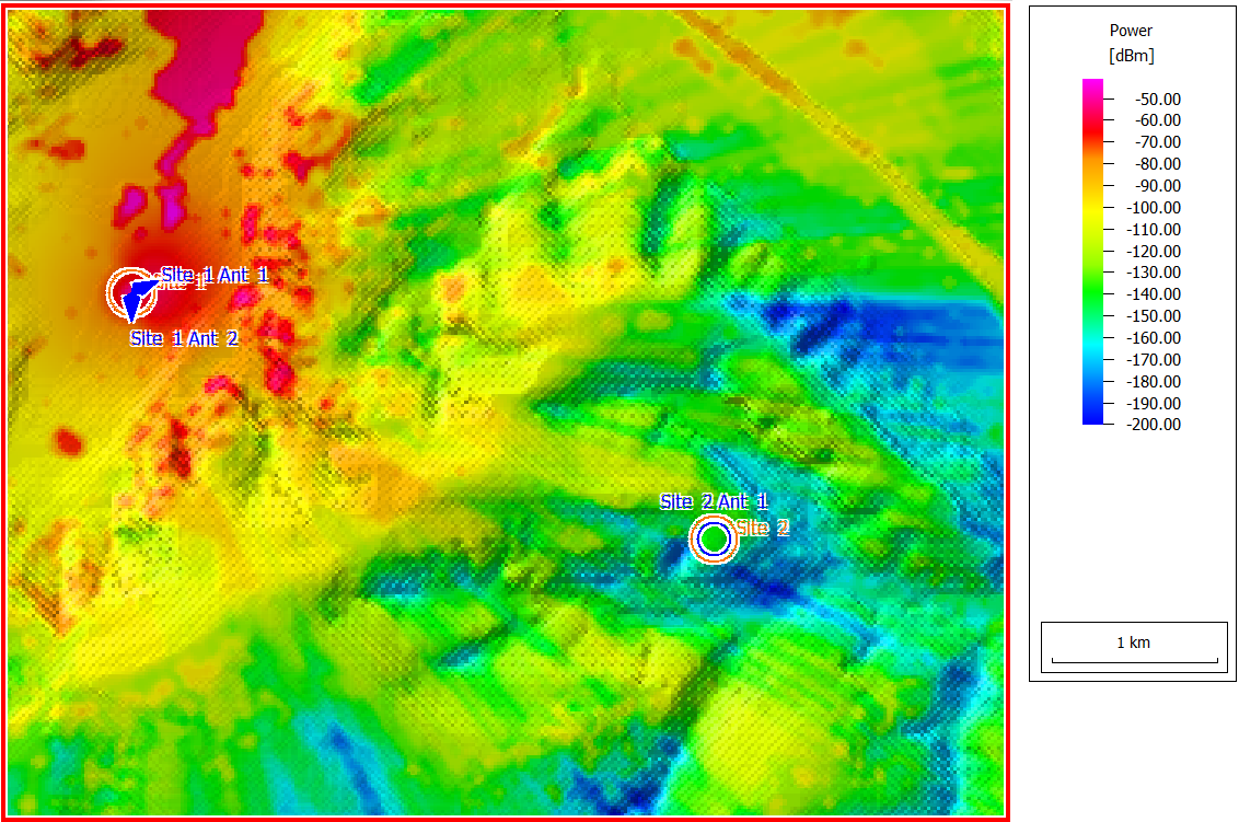
Figure 4. Power received from Power received from Site 1 Antenna 1.