OS-E: 0175 Continuum Shell Composites Using PCOMPLS
The PCOMPLS entry can be used to define continuum shell composites
using solid elements. Currently first order CHEXA and
CPENTA solid elements are supported.
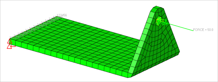
Figure 1. A Force is Applied on the RBE2 Element and the
Opposite End is SPC’d
Model Description
Conduct a continuum shell composite analysis of a bracket using PCOMPLS
entry. A force is applied on the RBE2 element and the other end of the
bracket is fixed at all degrees of freedom (Figure 1).
In addition to shell-based composites (via PCOMP,
PCOMPP, or PCOMPG), solid elements using
CHEXA and CPENTA elements can now be used to define
composite elements using the PCOMPLS entry. Multiple plies can be defined
on the PCOMPLS entry referencing corresponding materials, thicknesses,
and ply orientations. The current model under consideration consists of 7 plies with
different thicknesses and orientations. All plies reference the MAT9OR
material entry for orthotropic material entries.
FE Model
Elements Types
CHEXA
CPENTA
The linear material properties are:
MAT9OR
Young’s Modulus
E1=1.0E5
E2=5.0E3
E3=5.0E3
Poisson's Ratio
NU1=0.4
NU2=0.3
NU3=0.015
Results
The displacements and composite stresses can be seen in Figure 2. Figure 2. (a) Displacement; (b) Composite Stresses