Defining a response type 'Root Mean Square Deviation' for matching curve
Using the responses as objectives
Running the optimization and comparing the results in HyperGraph
Introduction
In this tutorial, you will reproduce the suspension optimization problem in
MV-3010 (Optimization using MotionView -
HyperStudy). The location (y and z
coordinates) of both inner tie-rod ball joint and outer tie-rod ball joint
are changed so that the toe vs. ride height curve matches a given desired
target curve.
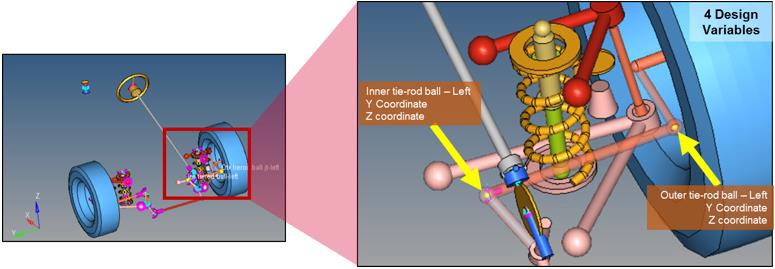
Figure 1. Suspension Topology to Optimize Figure 2. ‘Toe-ride height’ curve of initial design, optimized design and target design
You can compare the differences between MotionSolve
optimization and MotionView + HyperStudy optimization and learn the benefits of each
method.
Add Design Variables
In this step, you will add design variables for the optimization.
Before you begin, copy the file
mv_3023_initial_susp_opt.mdl and
target_toe.csv located in the
mbd_modeling\motionsolve\optimization\MV-3023 into your
<working directory>.
In MotionView, open
mv_3023_initial_susp_opt.mdl.
In the Project Browser, right-click on
Model and select Optimization
Wizard from the context menu.
Under Design Variable, click the Points tab.
All points listed are shown below.
Make the y and z coordinates of inner tie-rod ball joint and outer tie-rod ball
joint designable.
Go to point Otr tierod ball jt - left under the
Frnt SLA susp (1 pc LCA) system.
Expand the data member of it and select y and
z.
Click Add.
Under the Parallel steering system, add y and z data members to point
Inr tierod ball - left.
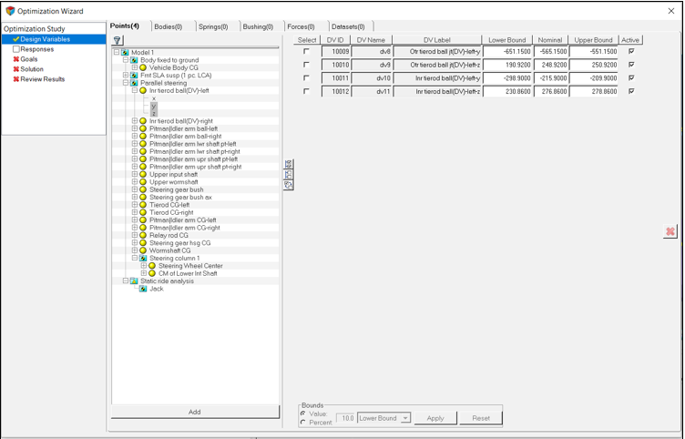
Change the upper and lower bounds of design variables according to
Table 1:
Table 1.
DV
Lower Limit
Upper Limit
Otr tierod ball jt(DV)-left-y
-651.15
-551.15
Otr tierod ball jt(DV)-left-z
190.92
250.92
Inr tierod ball(DV)-left-y
-298.9
-209.9
Inr tierod ball(DV)-left-z
230.86
278.86
The optimization wizard should look like the following image after
creating design variables:
Figure 3.
Add Response Variables
In this step, you will add response variables to the optimization.
The objective of the optimization is to make the toe vs. ride height curve match a
target design. The model already has the desired target curve defined and it will be
used in the response being created.
Click on the Responses page.
Click to add a response variable. Retain the default Label
and Variable name and click OK.
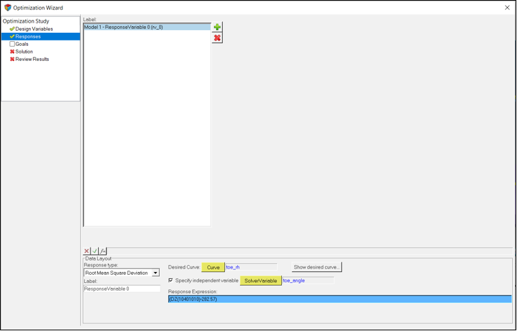
Once the response variable is created, under Response Type, choose
Response Type, Root Mean Square Deviation.
This response needs three user inputs:
Desired Curve - This is the target curve.
Response Expression - This is the value you measure.
Independent Variable - This defines the independent variable used to
calculate the target value.
For Desired Curve, click the Curve button and choose
toe_rh.
Activate the Specify independent variable check box.
Click SolverVariable to choose
toe_angle.
For Response Expression, enter the following expression for ride height:
`(DZ({MODEL.sys_frnt_susp.b_wheel.l.cm.idstring})-282.57)`.
You have finished creating the response. The user interface should appear as
it does in Figure 4: Figure 4.
Add Objectives and Constraints
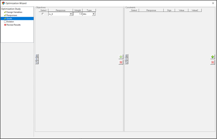
In this step, you will add an objective to the problem.
The objective in this problem is matching the toe ride height curve with the target
design. You can use the responses you created earlier in the tutorial as
objectives.
Navigate to the Goals page. Under Objectives, click
.
This will add an objective with the response rv_0. There are no
constraints in this problem, so the model is now ready to run. Figure 5. Defining objectives
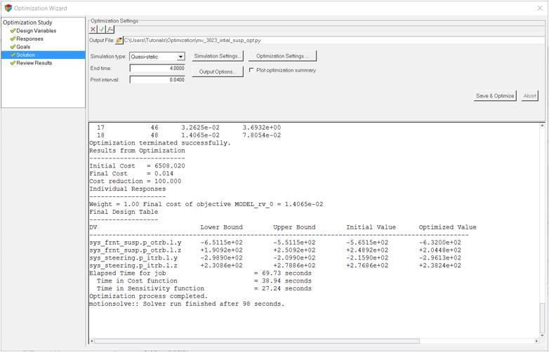
Run the Optimization
In this step, you will run the optimization.
Navigate to the Solutions page to specify optimization
settings and run the analysis.
Note: The model is saved before running, and if this is not desired, the model
can be saved with a different mdl file name before starting the
optimization. This can be done by closing the wizard, saving the model with
a different name and returning to the wizard again.
Accept all default optimization setting for this run.
Click Save & Optimize to run the optimization.
Figure 6. Solution Settings
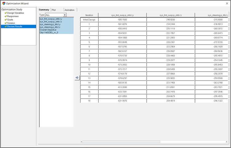
Post-Process
In this step, you will post-process the results of the optimization.
Once the optimization process is complete, review the result by clicking on the
Review Results page.
The summary window should look as shown in Figure 7: Figure 7.
You can also review the plots and animation by going to the Plot and Animation
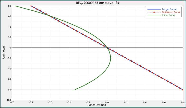
pages as we demonstrated in previous tutorials. For this optimization, it is
worthwhile to plot the toe – ride height curve for different iterations and see
how the curve approaches the target one.
Plot the toe-ride height curve for different iterations and see how it
approaches the target curve.
Close the Optimization Wizard.
Add an HyperGraph page to the
session.
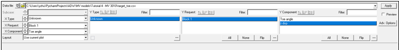
Open the file target_toe.csv.
In the plot panel, change the Type, Request, and Component of x and y
as shown in Figure 8.
Figure 8. Settings to plot target curve
You should see a straight line in the plotting
window.
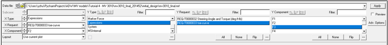
Navigate to the initial design folder and load the
.mrf file inside.
Change the Type, Request, and Component for x and y as shown in Figure 9.
Figure 9. Settings to plot initial design
Click Apply.
You should see a convex curve representing the 'toe-ride height' of the
initial design.
Go to the subfolder 'iter-18' (the last
iteration).
Import the .mrf file and plot the curve with the same
setting.
The 'toe-ride height’ curve of optimized design overlaps with the target
curve. Figure 10.
 to add a response variable. Retain the default Label
and Variable name and click OK.
to add a response variable. Retain the default Label
and Variable name and click OK.