HST-1535: HyperStudy Tutorial
HyperStudy tutorial.
Load Model in HyperMesh Desktop
In this step you will load the model.
-
In the Open Model dialog, open the
pipe.hm file.
A finite element model appears in the graphics area.
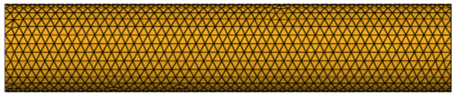
Figure 1.
Set Up AcuSolve Case
-
Create the material, Air_HM.
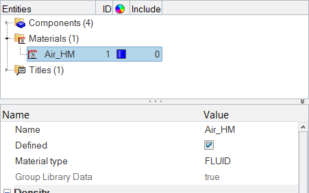
Figure 2. -
Modify the component, inflow.
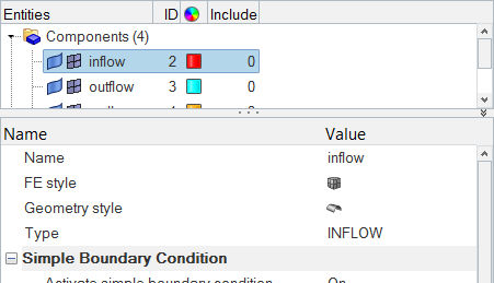
Figure 3. -
Assign a material to the component, fluid.
-
For Material, click Unspecified >>
Material.
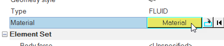
Figure 4.
-
For Material, click Unspecified >>
Material.
Morph Model
-
Create morph volume.
-
Click .
All of the elements in the model are selected.
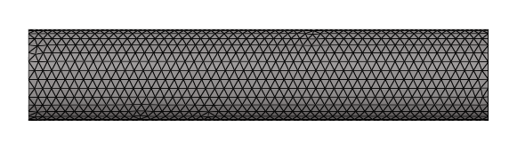
Figure 5. Selected Elements -
Click create.
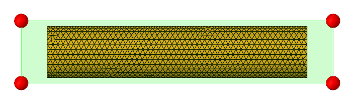
Figure 6. Morph Volume
-
Click .
-
Split morph volume.
-
In the graphics area, double-click on the edge of the model that is
marked by a green cross in Figure 7.
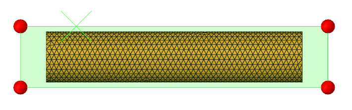
Figure 7. Morph Volume Split Edge
-
In the graphics area, double-click on the edge of the model that is
marked by a green cross in Figure 7.
-
Continue splitting the morph volume so that it resembles Figure 8.
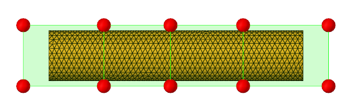
Figure 8. Morph Volume Split -
Repeat steps 5.d and 5.e for all of the edges until your model resembles the
following image.
Note: Verify that the yellow arrows are pointing in the correct direction along the edges.
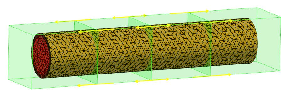
Figure 9. Updated Main-secondary Ends -
Morph the model.
-
In the dist = field, enter 0.010.
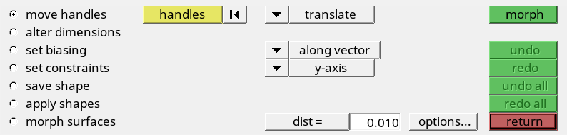
Figure 10. Settings for Move Handles Subpanel -
Select the four middle handles, highlighted in grey, in Figure 11.
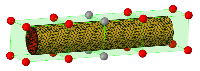
Figure 11. Middle Handles Selected -
Click morph.
The grid is morphed.
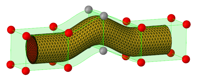
Figure 12. Morphed Grid
-
In the dist = field, enter 0.010.
-
Save shape.
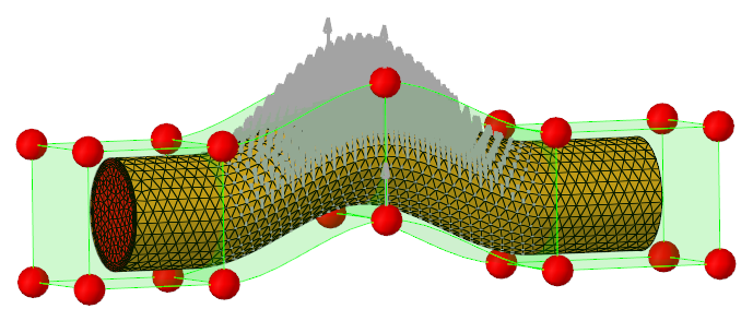
Figure 13. Saved Shape -
Show/hide shape.
-
In the Model Browser, right-click on the
Shape folder and select
Hide from the context menu.
The shape, s1 is hidden.
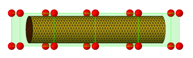
Figure 14. Shape Hidden -
Right-click on the Shape folder again and select
Show from the context menu.
The shape, sh1 reappears.
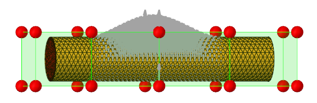
Figure 15. Shape Displayed
-
In the Model Browser, right-click on the
Shape folder and select
Hide from the context menu.
Perform Study with HyperStudy Job Launcher
-
On the CFD toolbar, click
 .
.
-
In the HyperStudy Job Launcher, set up and launch the
HyperStudy job.
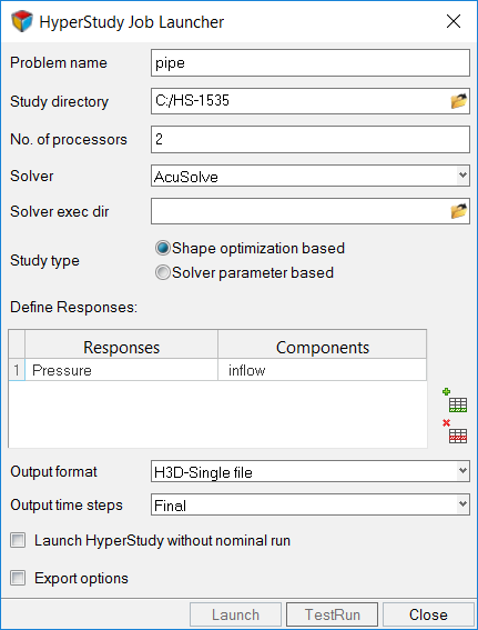
Figure 16. HyperStudy Job Launcher -
In the dialog that opens asking if you would like to continue, click
Yes.
A nominal run is submitted, and acuProbe and acuTrail are launched to provide you with updated information about the run. Once the run is finished, HyperStudy opens and with the study setup completed.
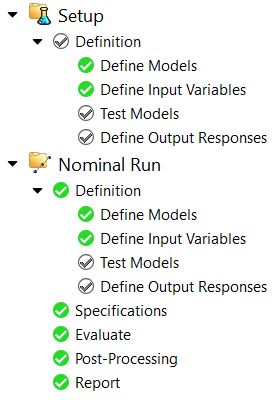
Figure 17. Study Setup
Run DOE
-
For bend, change Levels to 5.
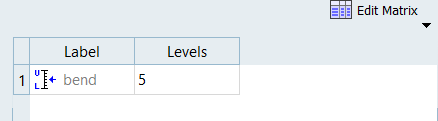
Figure 18. -
Plot the results of the inflow_pressure output response of the five runs.
- Click the Evaluation Plot tab.
- Using the Channel selector, select inflow_pressure.
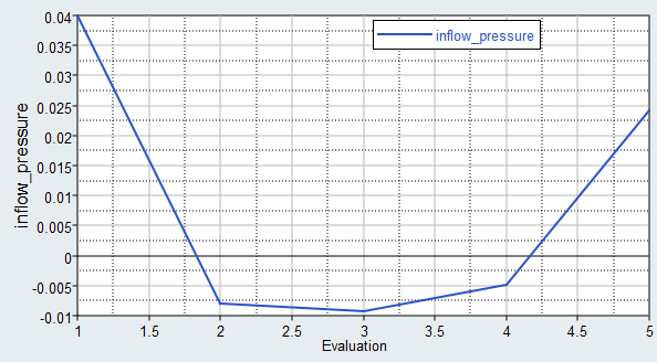
Figure 19. Evaluation PlotThe extreme left (bend = -1), middle (bend = 0) and extreme right (bend = 1) results correspond to the pipe shapes shown in Figure 20.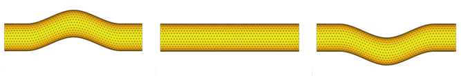
Figure 20. Pipe Shapes -
The results of the DOE can be visualized by loading the corresponding
*.h3d file from the run folder into HyperView.
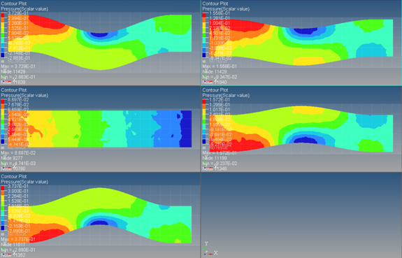
Figure 21. Contour Plot of DOE Results