Viewing the Results
View and post-process the results in POSTFEKO.
When you add excitations or loads to a solution, you unknowingly calculate the weighted sum of the various characteristic modes. Characteristic modes allow you to alter the behaviour of a structure without making any changes to the geometry.
-
Observe how the first characteristic mode can be recreated when sources are
placed in the appropriate locations.
Note: When comparing the characteristic modes to the reconstructed modes, all values need to be normalised.
- Plot the currents for the CharacteristicModeConfiguration1 (mode index = 1) in the 3D view.
- Plot the currents for StandardConfiguration1 in a second 3D view.
- Compare the currents for the first mode in CharacteristicModeConfiguration1 with the reconstructed mode using sources placed in the appropriate locations (StandardConfiguration1).
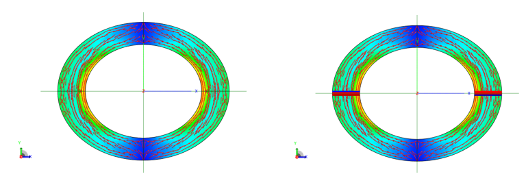
Figure 1. Compare the first characteristic mode of the MIMO ring (left) with the reconstructed mode (right). -
Observe how the fifth characteristic mode can be recreated when sources are
placed in the appropriate locations.
- Plot the currents for the CharacteristicModeConfiguration1 (mode index = 5) in a third 3D view.
- Plot the currents for StandardConfiguration2 in a fourth 3D view.
- Compare the currents for the fifth mode in CharacteristicModeConfiguration1 with the reconstructed mode using sources placed in the appropriate locations (StandardConfiguration2).
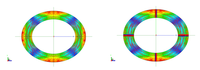
Figure 2. Compare the fifth characteristic mode of the MIMO ring (left) with the reconstructed mode (right). -
Compare the far fields of the characteristic modes configuration and the
reconstructed modes on a polar graph.
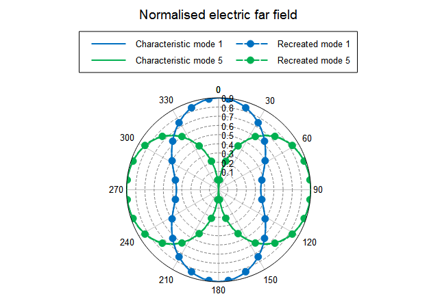
Figure 3. Comparison of the electric fields for the characteristic modes with the reconstructed modes.Note: Results are normalised in the comparison due to a lack of sources.The manually excited electric fields are in excellent agreement with the electric fields from the characteristic modes.