Intelligent Ray Tracing (IRT)
This unique model performs a rigorous 3D ray-tracing prediction which results in very high accuracy and due to the preprocessing of the database in very short computation time.
- The deterministic modeling of pathfinding generates a large number of rays, but only a few of them deliver the main part of the received electromagnetic energy.
- The degree to which visibility relations between walls and edges are independent of the position of the base station.
- The number of cases where neighboring receiving points are hit by rays for which the paths differ only slightly. For example, every receiving point in a street orthogonal to the street in which the transmitter is located is hit by a double reflected, single vertically diffracted ray and the points of interaction of these rays with walls and edges are independent of the receiver position (see Figure 1).
Based on these considerations it is possible to accelerate the time-consuming process of ray pathfinding by a single intelligent preprocessing of the database for buildings.
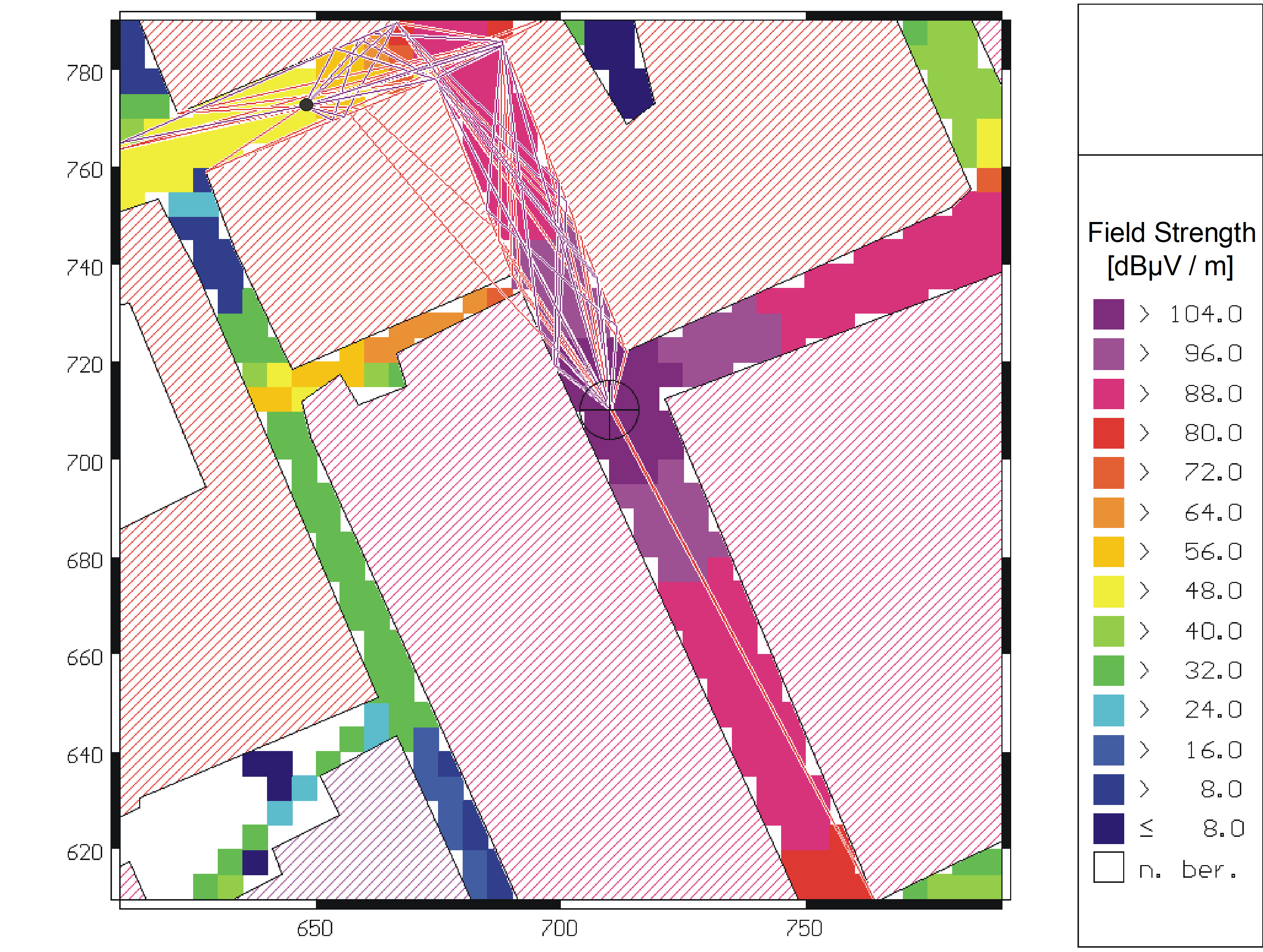
Figure 1. Rays between transmitter and receiver determined by ray-tracing.
Preprocessing
In a first step, as indicated in Figure 2, the walls of the buildings are divided into tiles and the edges into horizontal and vertical segments.
After this discretization of the database, the visibility relationships of the different elements are determined and stored in a file. For this process, all elements are represented and stored using their center positions. This leads to a simplification of the problem of ray pathfinding since possible interaction points are only determined by these the center positions of the tiles and segments.
The visibility relations between each tile (segment) and all other tiles (segments) are computed in preprocessing because they are independent of the transmitter and receiver locations.
For the decision about the visibility relations, the line of sight criterion between the center positions of the tiles (or segments) is evaluated. If there is a line of sight between the center positions, the rays from the center positions of the first tile to the corners of the second tile are determined. Then the projection of the angles of the rays on the first and second tile is stored together with the visibility relation.
A similar computation for the visibility relations between tiles and segments and between segments and other segments is performed and also stored in the preprocessing file.
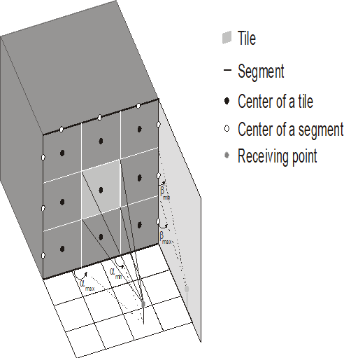
Figure 2. Subdivision of the building database into small elements.
The angles of the projection are very important because they define a range of possible reflection (or diffraction) angles for the illuminated tile (or segment). The angle also continues onto the neighboring tile resulting in a very accurate prediction of the rays even if the tiles or segments are large - up to 50 or 100 meters for urban databases (Hoppe1).
A further improvement is possible if the grid of the prediction points is also used in the preprocessing because the prediction plane can be subdivided into tiles and the visibility relations between the tiles of the prediction grid and the tiles (and segments) of the walls represent the last part of the ray in the direction to the receiver.
If the receiver visibility relations are determined in the preprocessing, the only remaining visibility relations to be computed in the prediction are the ones from the transmitter to the tiles (of walls and prediction grid) and segments. Figure 2 depicts the visibility relations between a tile and a receiving point. For the calculation of the angles, the connecting straight lines between the receiving point and the four edges of the tile are considered.
By projecting these four lines onto the XY plane and additionally into a plane perpendicular with respect to the inspected wall, four angles are determined which give an adequate description of this visibility relation.
Memory Requirement and Computation Time
Table 1 shows the memory requirements for the preprocessed database file and computation times for different urban scenarios. They were all computed with a maximum extension of the tiles and segments of 50 meters and a prediction resolution of 10 meters.
| Example | Area [km2] | Number of Buildings | File Size [MB] | Relative Computation Time |
|---|---|---|---|---|
| Munich | 8 | 2000 | 50 | 100% |
| Stuttgart | 4 | 300 | 18 | 4% |
| Lille | 1 | 86 | 6 | 0.6% |
These computation times are shorter than the computation times of a single prediction for the same area using the standard ray-tracing because each visibility relation is only computed once in the preprocessing while in the prediction with standard ray tracing similar visibility relations might be considered and computed for many prediction points.
Prediction
The result of the preprocessing of the building database is a tree structure containing tiles, segments and receiving points of the prediction area, for example, as indicated in Figure 3. In this tree, every branch symbolizes a visibility relationship between two elements.
For the prediction only the tiles, segments and receiving points, which are visible from the base station, have to be determined. Also, the angles of incidence for the visible tiles and segments have to be calculated. Subsequently, pathfinding can be done similar to the ray launching algorithm by recursively processing all visible elements and checking if the specific conditions for reflection or diffraction are fulfilled. The ray search is stopped if a receiving point or a given maximum number of interactions is reached. Finally, the field strength is summed up at all potential receiving points.
Figure 3 shows the arrangement of all visibility relations computed in the preprocessing and the prediction.
The preprocessing of the building database reduces the time-consuming process of pathfinding to the search in a tree structure. A comparison between the number of branches in the first layer (determined in the prediction) with the number of branches in the remaining layers (determined in the preprocessing) in the tree structure given in Figure 3 indicates the relation between the computational effort in the prediction and the computational effort in the preprocessing.
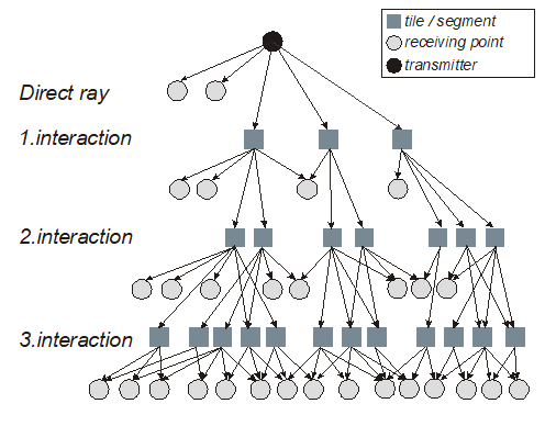
Figure 3. Determination of ray paths by searching in a tree structure.
Due to the small number of visibility relations in the first layer of the tree, the computation times are very short. Most of the time is spent on reading the visibility data from a file. If more than one transmitter is considered at the same time, the preprocessed data must only be read once and thus the prediction of the second transmitter is even faster than the prediction of the first transmitter because the visibility tree is already loaded into memory.
Low Dependency of Prediction Area
The computation time for the prediction is nearly independent of the size of the prediction area because the whole tree is computed once for each prediction and all receiver points are included in the prediction. Only the time for computing the field strength is necessary for the evaluation of a prediction point and this time depends on the location of the point (inside or outside the prediction area). The rays to all preprocessed receiver points are always determined in each prediction.
Therefore if the size of the prediction area is reduced, a smaller number of prediction points must be considered (more preprocessed prediction points are neglected) and the time for computing the field strength is reduced. But this part of the computation time is very short compared to the time for determining the rays and therefore the total computation time is nearly independent of the size of the prediction area. The number of interactions influences the computation time because each new interaction corresponds to a further layer in the visibility tree.
Results
Very good results are achieved with a maximum number of three interactions (reflections and multiple diffractions in different combinations with a maximum number of two diffractions in each ray).
Table 2 shows the computation times for the different urban scenarios using intelligent ray-tracing. The computation times are compared to the ones of an accelerated 3D standard ray-tracing model.
| Example | Area km2 | Number of Buildings | Relative Time, IRT | Relative Time, SRT |
|---|---|---|---|---|
| Munich | 8 | 2000 | 0.3% | - |
| Stuttgart | 5 | 300 | 0.05% | 100% |
| Lille | 1 | 86 | 0.006% | 20.8% |
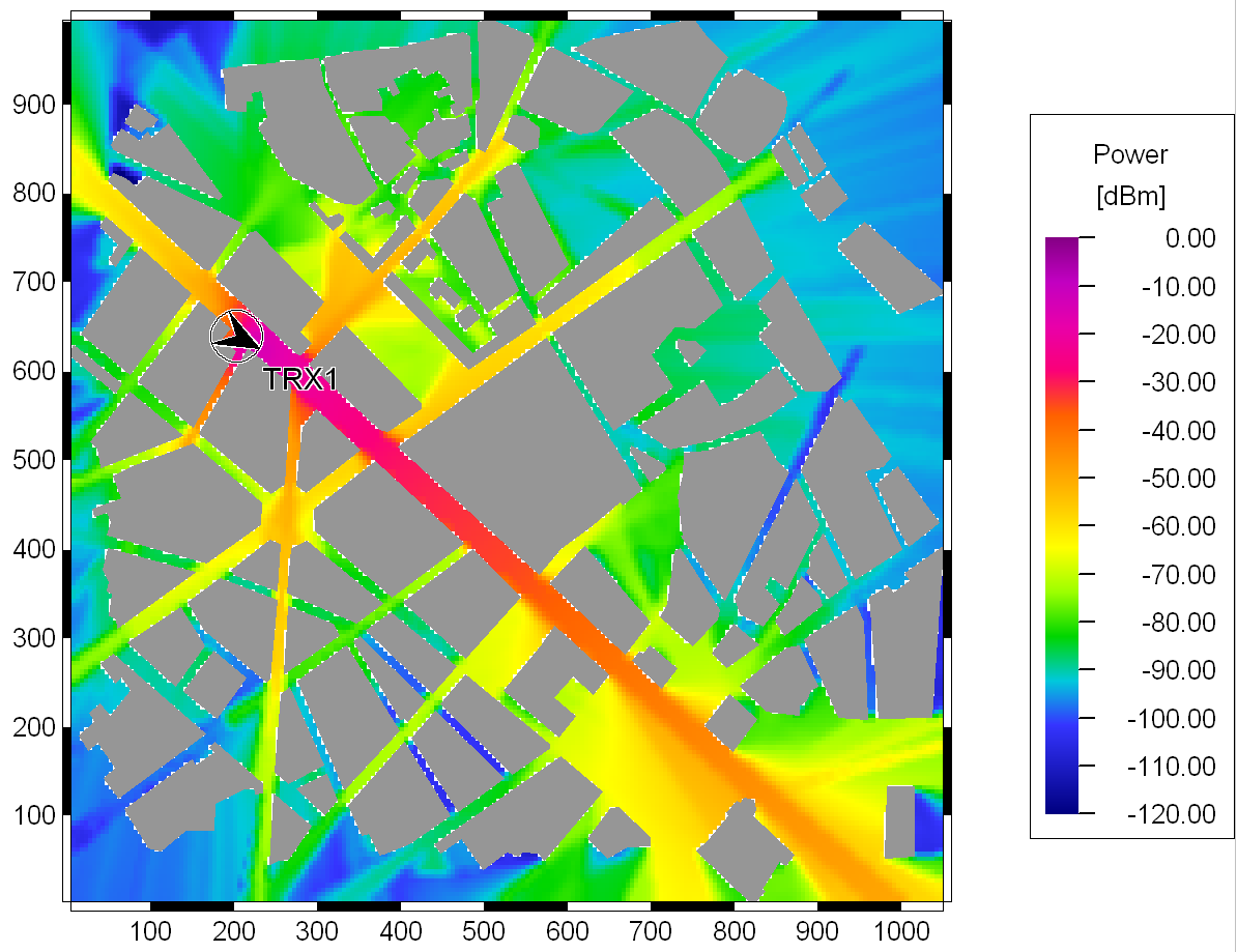
Figure 4. Prediction of the received power with intelligent ray-tracing.
A comparison of this prediction with preprocessing of the database on the one hand with a prediction calculated with the standard 3D ray-tracing, on the other hand, leads to very small differences.
2 x 2D Modeling
From the many transmitter-to-receiver propagation paths, the most dominant ones have to be selected to obtain the total received power with moderate computation time. A useful acceleration of the process of ray pathfinding under the consideration of the main propagation mechanisms is the limitation to two orthogonal planes (double 2D). Rooftop diffracted paths are included in the vertical plane approach, while for buildings the diffracted paths are modeled with the transverse plane approach as depicted in Figure 5. The propagation in both the vertical and the transverse plane is considered in two dimensions. However, the determination of the building corners in the transverse plane is not necessarily performed in a horizontal plane. This principle can also be considered for the intelligent ray-tracing approach which leads to the following two 2 x 2D models included in ProMan:
- 2x2D (2D-H IRT + 2D-V IRT)
The preprocessing and the determination of propagation paths are done in two perpendicular planes. One horizontal plane (for the wave guiding, including the vertical wedges) and one vertical plane (for the over rooftop propagation including the horizontal edges). In both planes, the propagation paths are determined similarly to the 3D-IRT by using ray optical methods. This approach neglects the contributions from reflections at the building walls which are in most cases only relevant for the streets with LOS to the transmitter.
- 2x2D (2D-H IRT + COST231-W-I)
This model treats the propagation in the horizontal plane in the same way as the previously described model, thus by using ray-optical methods (for the wave guiding, including the vertical wedges). The over rooftop propagation (vertical plane) is taken into account by evaluating the COST 231-Walfisch-Ikegami model. By using this model, only the propagation in the horizontal plane is determined by ray-optical methods taking into account the vertical wedges of the buildings, while the over rooftop propagation is modeled by an empirical approach.
Due to the restriction to two orthogonal planes, this approach has better computational performance but at the cost of a slightly reduced accuracy - not all buildings are taken into account for the determination of ray paths.
Figure 5. Ray tracing within a vertical and a transverse transmitter-receiver plane.