Calibration of Models
WinProp allows the automatic calibration of nearly all available propagation models based on measurement data.
Calibration of Propagation Models
WinProp allows the automatic calibration of nearly all available propagation models based on measurement data. Additionally some propagation models support the calibration of material properties and of clutter/land usage databases. The following table shows an overview of the models and the features.
| Scenario | Model | Material calibration | Clutter calibration |
|---|---|---|---|
| Indoor | One slope model | no | not applicable |
| Motley-Keenan model | no | not applicable | |
| COST 231 model | yes | not applicable | |
| Dominant path model | no | not applicable | |
| Standard ray-tracing | yes | not applicable | |
| Intelligent ray-tracing | yes | not applicable | |
| Urban | Knife edge model | no | not applicable |
| Dominant path model | no | not applicable | |
| Intelligent ray-tracing | no | not applicable | |
| Rural | Empirical two ray model | not applicable | yes |
| Deterministic two-ray model | not applicable | yes | |
| Dominant path model | not applicable | no |
The following picture shows the procedure for the calibration of the propagation models:
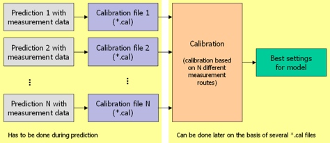
Figure 1. Procedure for calibration of propagation models.
As shown in the picture, during the prediction calibration files are written to the hard disk. The calibration is done afterwards based on the calibration files (.cal). The steps for the calibration are explained in the following sections.
Generation of WinProp Measurement Files
Measurement files in WinProp file format (.fpp, .fpl, .fpf) have to be created prior to the calibration. This means the raw measurement data has to be imported from simple ASCII files into the WinProp software. See Import Prediction Data for more information.
Assignment of Measurement Files to Transmitters
to retrieve a calibration file (.cal) after the prediction, a measurement file has to be assigned to the corresponding transmitter. Only one measurement route can be assigned to one transmitter. In the picture below it is shown how a measurement file can be assigned to a transmitter.
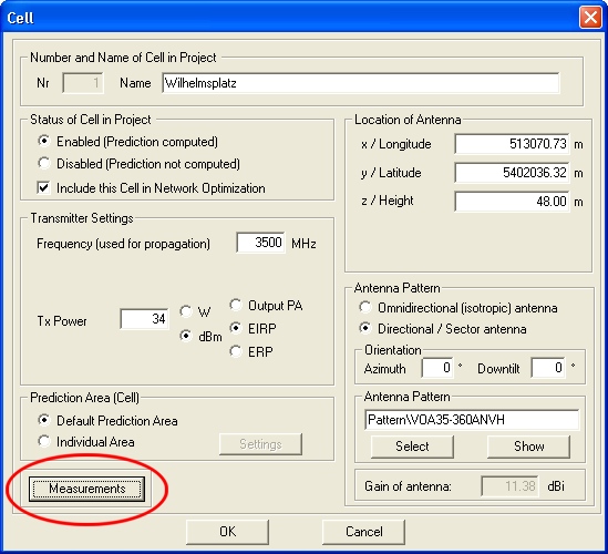
Figure 2. The Cell dialog.
The button indicated with the red circle is used to assign a measurement file (.fpp, .fpl, .fpf files are supported) to the selected transmitter. The measurement file must contain measured data from the selected transmitter only. Superposed measurement data from several transmitters is not supported. When the measurement data is in path loss format (.fpl) cable loss must not be included. In contrast to this, cable loss is expected as “included” when measurement data is available in field strength or power file format. Antenna gain is always expected as “included”.
Computation of Propagation Prediction
After the assignment of the measurement files to the transmitters is completed, the wave propagation prediction can be launched as usual. The propagation paths output needs to be activated, otherwise no .cal files will be generated.
For each transmitter (with measurement data assigned) a calibration file (.cal) is written to the hard disk. If the files are missing, click the Prediction tab, under Additional Prediction Data... and select the Propagation Paths check box.
Calibration Computation
The calibration tool can be started from the Computation menu (). The calibration files generated during the wave propagation prediction have to be added to the list. This is shown in the image below.
The Calibration dialog
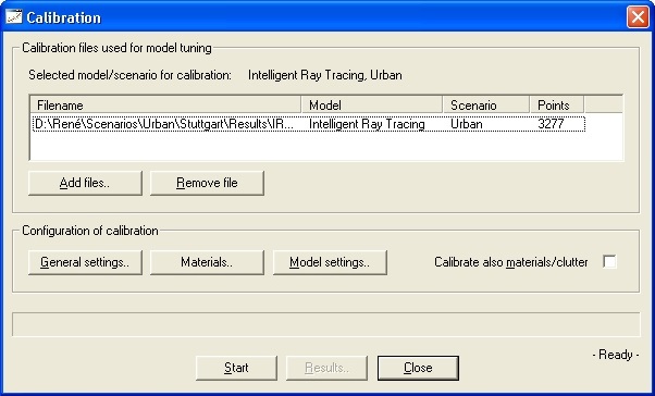
Files can be added by clicking on Add files. They can be deleted by clicking on Remove file.
The settings can be adapted to the users needs by selecting General settings. This allows you to influence the selection of the measurement points, thus only points in a given power (dBm), path loss (dB) or distance (m) range will be considered.
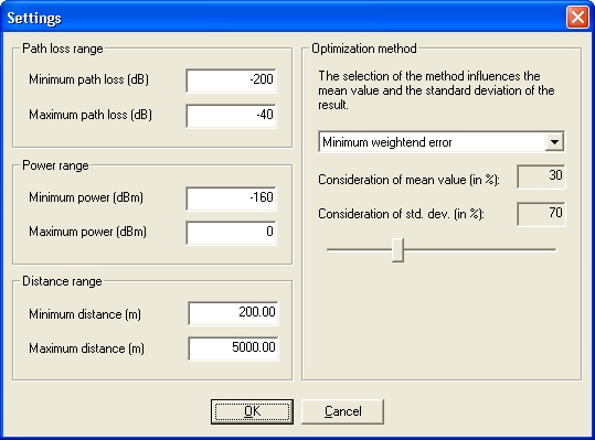
Figure 3. The Settings dialog.
- Minimum mean error
- The goal of the optimization is to achieve a minimum mean error (nearest to zero). The standard deviation is not considered and thus might be larger.
- Minimum mean squared error
- The goal of the optimization is to achieve a minimum mean aquared error. The standard deviation is not considered and thus might be larger.
- Minimum standard deviation
- The goal of the optimization is to achieve a minimum standard deviation. The mean error is not considered and thus might be larger
- Minimum weighted error
- The goal of the optimization is to find the best combination of minimum mean error and minimum standard deviation. The weighting between mean error and standard deviation can be adapted by the user.
The range of the model parameters can be defined in the Model settings dialog. As larger the range is, as longer the calibration will take. The model parameters depend on the selected propagation model, thus each model offers individual model parameters. The following screenshot shows model parameters for the Urban Intelligent Ray Tracing.
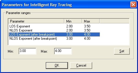
Figure 4. The Parameters for Intelligent Ray Tracing dialog.
Depending on the propagation model the material database or the clutter/land usage database can be calibrated additionally.
After clicking Start, the calibration begins and the progress is shown with a progress bar. In some cases the calibration process does take up to one hour.
Calibration Result
After a calibration has finished the results are displayed in a table. The picture below shows the results for the urban Dominant path model. Depending on the propagation model different parameters are listed in the table.
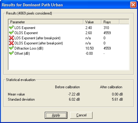
Figure 5. The Results for Dominant Path Urban dialog.
The model parameters listed in the table can now be transferred manually into the project settings of ProMan and the project can be recomputed to achieve better results based on the new model parameters. By clicking on Apply the material properties (as far as they have been calibrated) are applied to the vector/material database.
The message box shown above gives also information about mean value and standard deviation from measurements to predictions before and after the calibration. Depending on the optimization method different results can be obtained.