Use the View Data tab to specify, plot and view your data. The tab is divided into
three working sections: Dynamic Data, Static Data, and Curve and Plot Properties. A fourth
section displays a static image of the Conceptual Cubic.
Use the Dynamic Data area of the tab to define the display
layout for dynamic stiffness and loss angle measurements.
Click the For each, Then for
each and Show data for each files
fields to determine the sorting of your data by direction, amplitude and
preload.
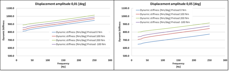
For each direction, data for a specific amplitude is displayed in a
plot window. In each plot window several curves are drawn—one for each
preload. Each curve is the graphical representation of the dynamic
stiffness (loss angle) vs. frequency relationship.
Click the Separate plots for dynamic stiffness & loss
angle to specify whether the dynamic stiffness and loss
angle are to be plotted in the same window or in separate windows
(default).
Use the Static Data area of the tab to determine how to
display the static properties derived from the experimental measurements. The
tab includes three representation options for the static data.
The Spline Data section uses data obtained from the static testing of
the physical bushing that is stored in the .spd
file.
The Constant Stiffness area displays the linear fit to the spline data.
The slope at the operating point, OS, is used to represent the bushing
stiffness in that direction. Note that constant damping as a default is
assumed to be 1% of the constant stiffness.
The Conceptual Cubic area defines the cubic polynomial that approximates
the spline data. For more information, see Features of the Altair
Bushing Model and refer to sections on Stiffness Force
Models, Damping Force Models, and the
Bushing Property File (.gbs).
Use the Curve and Plot Properties options to define the
line-style and line-thickness for dynamic stiffness and loss angle curves. The
default option is a line-style and coloring scheme that shows the most contrast
between the curves.
Click Common axis range for curve plots to
specify that all plots for dynamic stiffness or loss angle use a common
range for the x- and y-axes. Using the same axis range is useful for
visually examining the curves.
Note: If the option is not selected, the HyperWorks
determines the range for each plot, which is useful when you need
more detail. In addition, HyperGraph
lets you manually zoom in and out on the curves.
Click Start y-axis at zero to specify that all
plots for dynamic stiffness or loss angle start with a y-value of zero.
This option is useful when you want to zoom out and visualize experiment
and model behavior on an absolute scale.
Use the series of four buttons at the bottom of the View Data tab to do the
following:
Click Save Settings to save the dynamic data,
curve, and properties preferences for reuse.
Click Load Settings to load previously saved
preferences for dynamic data and curve and plot properties.
Click Append Plots to append new curves to an
existing HyperGraph session.
Click New Plots to clear the HyperGraph session and plot new curves for
dynamic and static data.
Dynamic Data
Dynamic data is plotted according to the scheme you define in
the Dynamic Data section of the View Data tab. The following sample plots show Dynamic
Stiffness vs. Frequency for various amplitudes for the FX direction: Figure 1.
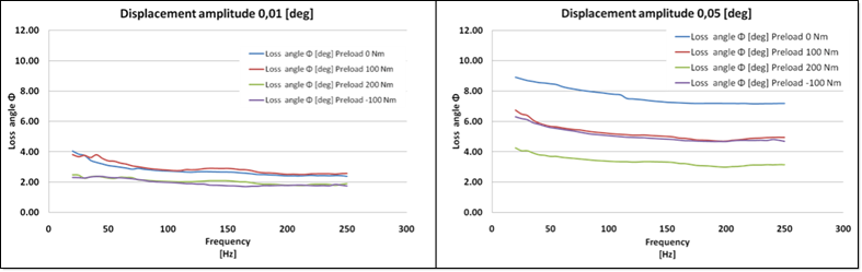
The following are sample plots for Loss Angle vs. Frequency for various
amplitudes for the FX direction. Figure 2.
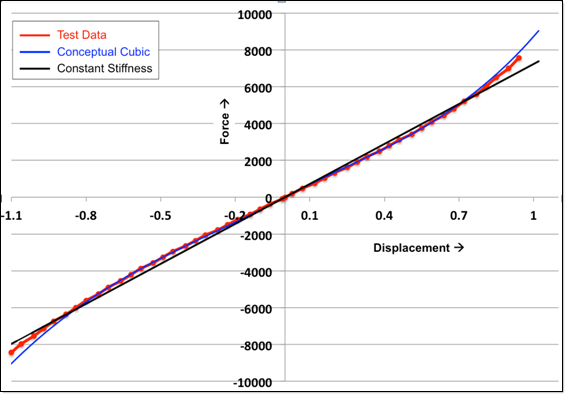
Static Data
Following are two plots for static data. Each plot
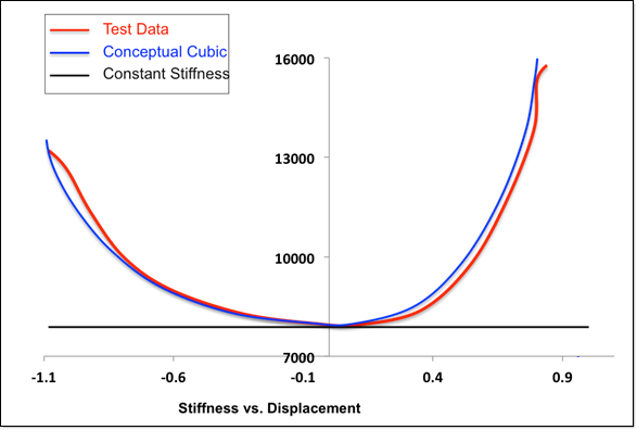
contains three curves: the red curve indicates experimental data, the blue curve
indicates the conceptual cubic, synthesized from the static data, and the black
curve indicates constant stiffness.
The following plot shows the Force vs.
Displacement behavior for the three curves: Figure 3.
The following plot shows the Stiffness vs. Displacement behavior of the
bushing. Figure 4.