In this tutorial, you will analyze a friction stir welding of a butt joint. This example shows you how to set up the data for HyperXtrude and solve the problem.
The model files for this tutorial are located in the file mfs-1.zip in the subdirectory \fsw\FSW_0020\. See Accessing Model Files.
To work on this tutorial, it is recommended that you copy this folder to your local hard drive where you store your HyperXtrude data, for example, “C:\Users\HyperWeld\” on a Windows machine. This will enable you to edit and modify these files without affecting the original data. In addition, it is best to keep the data on a local disk attached to the machine to improve the I/O performance of the software.
Process
The process for analysis using FSW is as follows:
| 1. | Select the units for the analysis. |
| 2. | Create data files for butt weld joint. |
| 3. | Mesh the computational domain. |
| 4. | Assign material properties and process conditions. |
| 6. | Visualize the model in HyperXtrude and inspect material and bc’s. |
| 7. | Launch HyperXtrude. HyperXtrude can also be started from the command line |
| 8. | Post-process the results in HyperXtrude. |
Exercise
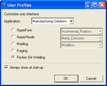
Step 1: Load the FSW user profile
| 2. | From the Preferences menu, click User Profiles. |
| 3. | For Application, select Manufacturing Solutions. |
| 4. | Select Friction Stir Welding. |
Step 2: Select units
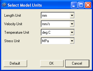
| 1. | On the Utility Menu, click Select Units. |
A window displays with the option to select units for length, velocity, temperature, and stress.
| 2. | Select the units to use and click OK. |
Step 3: Create the butt weld model
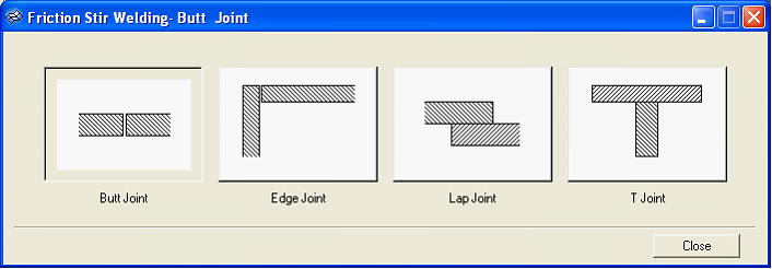
| 1. | On the Utility Menu, click Create Mesh. |
The Create Weld Joint window with icons showing available parametric model’s weld joints display.
The geometric parameters for the butt weld joint displays. A weld joint is defined by the length, width, and thickness of the plate geometry. Pin diameter, pin height, shoulder diameter, and shoulder height are used to define the tool geometry.
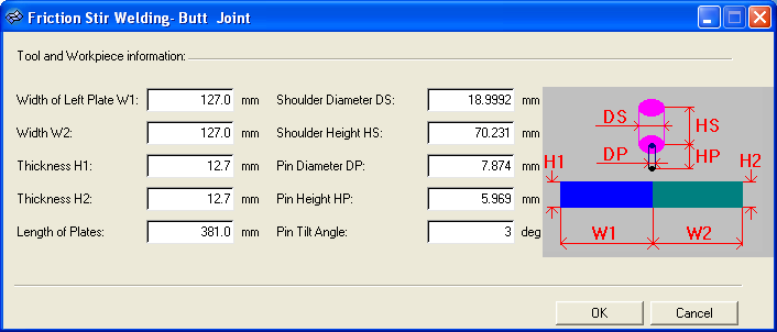
| 3. | Review the default data, and click OK to create the mesh and continue to the Process Parameters window. |
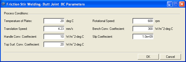
| 4. | Click OK to accept the default values. |
The process parameters are inputted into this window. The process parameters include: temperature of plates, rotational speed and translational speed of the tool, friction coefficient at the shoulder contact surface, convective heat transfer coefficient, and the ambient temperature.
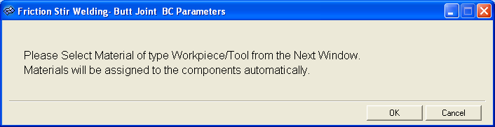
| 5. | Continue to select material properties. |
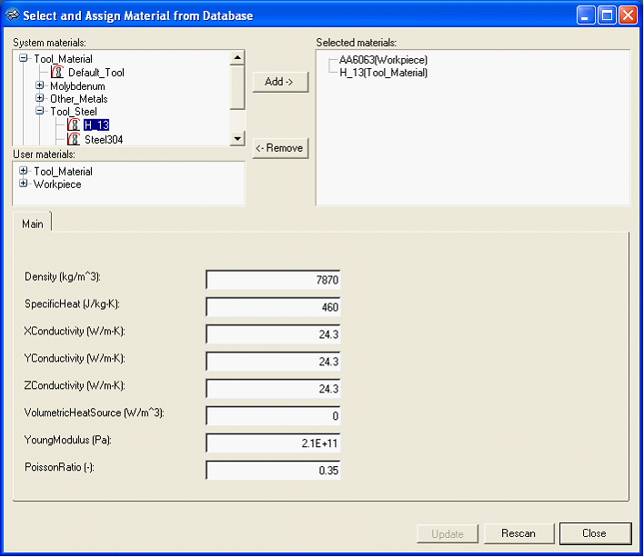
| 6. | Under System Materials, select H-13 and AA6063. |
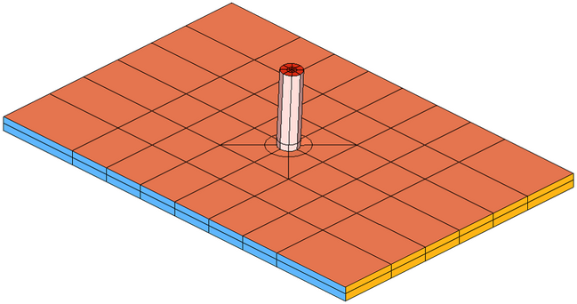
The mesh generation process completes. The finite element mesh of the weld joint with boundary conditions displays in the main graphics area.
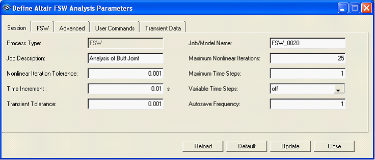
| 8. | On the Utility Menu, under Process Data, click Parameters. |
The first property page on the parameters widget displays the job control parameters. The second page contains the process parameters. The third page contains the advanced parameters such as the nonlinear iteration relaxation parameters. The last page allows you to enter additional run control commands.
| 9. | Change the Job/Model Name to FSW_0020 and click Update. Click Close to close the dialog. |
Step 4: Summarize the model
| 1. | On the Utility Menu, under Process Data, click Model Summary. |
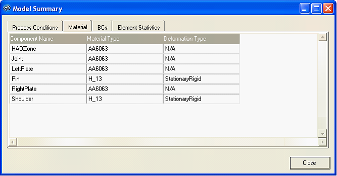
The information on the mesh size, type of elements, boundary conditions, and materials displays.
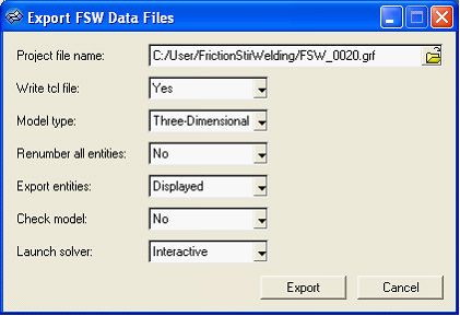
Step 5: Export data files
Next you will save the mesh, material properties, boundary conditions, and process conditions in HyperXtrude solver data file format.
| 1. | On the Utility Menu, under Export Data, click FSW. |
| 2. | Use the browser window to select the directory to store data files. |
| 3. | Save the file as fsw_0020.grf. |
Step 6: Load the model to HyperXtrude
| 1. | Using a command window, go to the location of your work directory. |
| 2. | At the command prompt, type %hx –I butt_joint.tcl. |
HyperXtrude launches and loads the tcl file.
| 3. | Click View to launch the main viewport where the geometry is displayed. |
Step 7: Inspect materials and process parameters
| 1. | From the Properties menu click Material. |
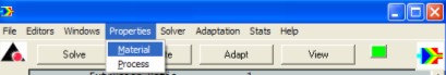
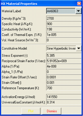
A form containing the material properties of aluminum displays.
| 2. | Verify that the material properties are the same as the ones given in butt_joint.grf. |
| 3. | Click Plot to view the plot of temperature and strain rate dependent viscosity and flow stress. |
| 4. | From the Properties menu, click Process. |
A form displaying the reference quantities opens.
Step 8: Open the main viewport
| 1. | From the Windows, menu click Status. |
| 2. | Click View to view the main viewport. |
Step 9: Change the background color
| 1. | Click the mesh icon  . . |
| 2. | Select the Graph Opts panel from the Viewport Control Form. |
| 3. | Select Background: white. |
Step 10: Inspect the boundary edges
| 1. | Click on the BC icon  . . |
| 2. | Click Update to get a list of all the different BCs. |
| 3. | Display the boundaries by selecting one at a time and then click the Redraw button. |
| 4. | Turn off the mesh and Dismiss the Viewport Control Form. |
| 5. | Deselect all the boundaries and Dismiss the Data View Form. |
Step 11: Inspect the mesh
| 1. | Leave the boundaries displayed. |
| 2. | Select Grid panel from the Viewport Control Form. |
| 3. | On the Mesh menu, click Full. |
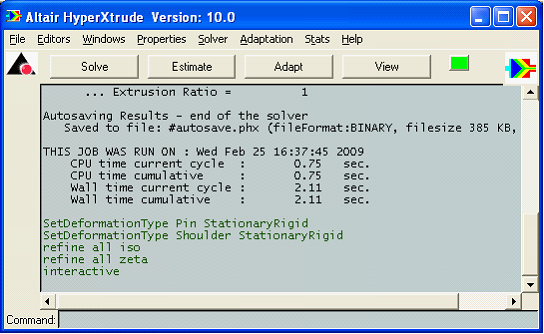
Step 12: Run the analysis
| 1. | Click Solve. This starts the HyperXtrude analysis. |
The Ready (displayed in green) button will turn red indicating that the code is busy computing.
| 2. | Observe the run diagnostics on the screen and wait till the Ready button turns green again. |
The solution process stops after 25 nonlinear iterations.
Step 13: Post-process the results
| 1. | Click the Load Results icon  . . |
This step loads nodal values of all of the results for post-processing. You can also selectively load what you require to optimize the memory requirements.
Step 14: Display color plots of the results
| 1. | Click the Isosurfaces icon  . . |
| 2. | Choose Display: flat and click Apply. The pressure solution is shown. The pressure in the solid domain is equal to zero. |
| 3. | Change Color by to Velocity Magnitude. |
| 4. | Change Color by to Temperature. Due to the differences in thermal properties of the two materials, the shapes of the temperature contours in two regions are different. |
Step 15: Display particle traces
| 2. | Click Select-all to show all BC faces. |
| 3. | In the Color bar widget, turn off the color bar. |
| 4. | Click the Particle Traces icon  . . |
| 5. | Select the Traces page from the Data View Form. |
| 6. | Select Traces Start From: Inflow. |
| 7. | Click Launch. The particle traces are displayed |
Step 16: Display velocity vectors
| 1. | From the Data View form, select the Vectors page. |
| 2. | Set Scale= 10 and enable the check box Color by magnitude. |
| 3. | Click Apply. The velocity vectors are displayed. |
| 4. | Clear the Show check box to turn off the display. |
| 5. | Dismiss the Data View Form. |
Return to Friction Stir Welding Tutorials


