HL-T: 1100 Stress Life (S-N) Using Stress History Created from Modal Participation Factors (via a *.pch file) and Modal Stress
In this tutorial you will:
- Import a model to HyperLife
- Select the SN module with a Modal Superposition loading type and define its required parameters
- Create and assign a material
- Assign a *.pch file (containing modal participation factors) to modal stresses
- Evaluate and view results
Before you begin, copy the file(s) used in this tutorial to your
working directory.
- HL-1100\Rear_Truss.h3d
- Rear_Truss_modal.pch
Note: The aim of this tutorial is to:
- Create stress history from modal participation factors and modal
stresses.For the complete time interval, stress history is given by:Where,
- Stress history for the given time interval of an element
- Participation factor per mode at time t (via mrf/pch file)
- Modal stress of an element per mode (via h3d file)
- Mode
- Perform an SN uniaxial calculation for the above stress history.The above pch file is generated from OptiStruct from a modal transient run.
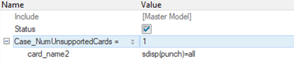
Figure 1.
Import the Model
-
From the Home tools, Files tool group, click the Open Model tool.

Figure 2. -
Click Apply.
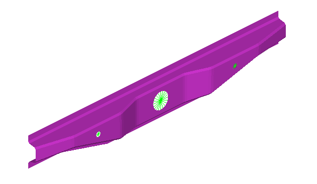
Figure 3.
Tip: Quickly import the model by dragging and
dropping the .h3d file from
a windows browser into the HyperLife
modeling window.
Define the Fatigue Module
-
Click the SN tool.
The SN tool should be the default fatigue module selected. If it is not, click the arrow next to the fatigue module icon to display a list of available options.

Figure 4.The SN dialog opens. -
Define the SN configuration parameters.
- Select Uni Axial as the method.
- Select MPa for the FE model units.
- Select Abs Max Principal for the stress combination
- Enter a value of 0.5 for the certainty of survival.
- Select GOODMAN for the mean stress connection.
- Select Worst for the layer selection.
- Select Modal Superposition for the type of loading.
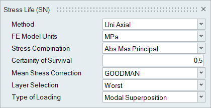
Figure 5.
Assign Materials
-
Click the Material tool.

Figure 6.The Assign Material dialog opens. -
Create a new material.
-
Click
 to create a new material.
-
Accept all other default settings then click Plot &
Save.
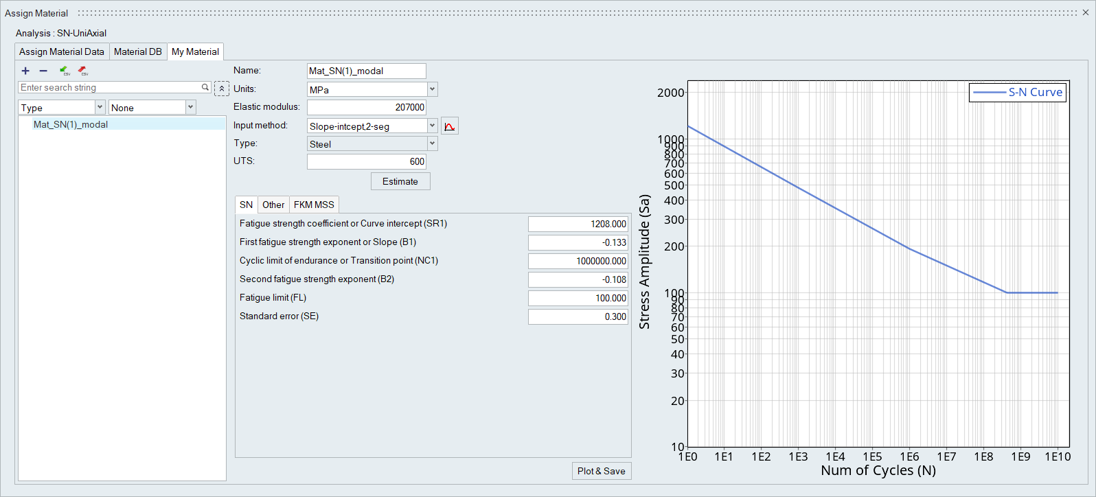
Figure 7.
-
Click
-
Return to the Assign Material Data tab and select
Mat_SN(1)_modal from the Material drop-down menu for
Rear_Truss_1.
The Material list is populated with the materials selected from Material Database and My Material.
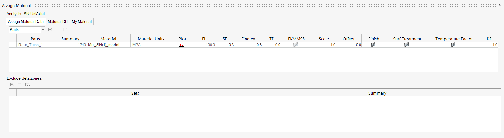
Figure 8.
Assign Load Histories
-
Click the Load Map tool.

Figure 9.The Load Map dialog opens. -
Click
 in the Choose File field and
browse for Rear_Truss_modal.pch.
in the Choose File field and
browse for Rear_Truss_modal.pch.
-
Click
 to add the modal participation file.
-
On the bottom half of the dialog, click .
ModalEvent_1 is created with 1 repeat.
-
Activate the ModalEvent_1 checkbox.
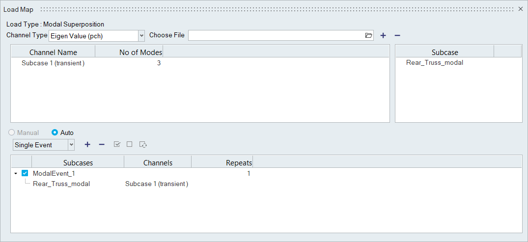
Figure 10.
Evaluate and View Results
-
From the Evaluate tool group, click the
Run Analysis tool.

Figure 11.The Evaluate dialog opens.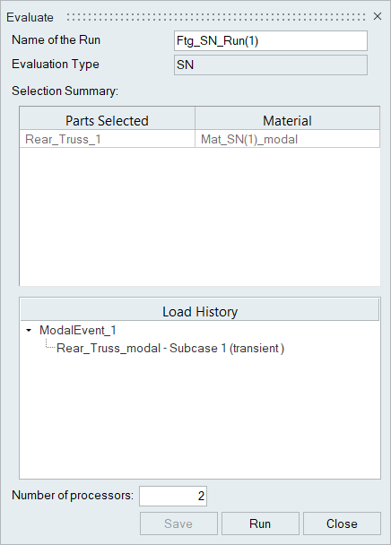
Figure 12. -
Use the Results Explorer to
visualize various types of results.
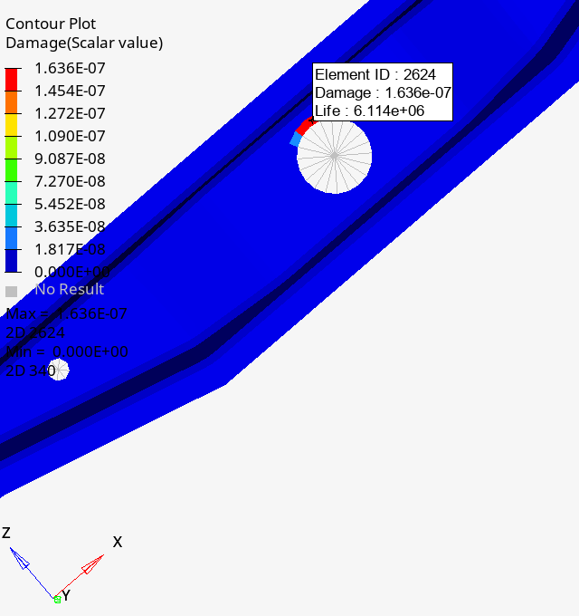
Figure 13.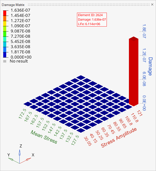
Figure 14.