HL-T: 1070 Transient Stress-Life (S-N)
During Transient Fatigue Analysis, the load-time history input is not required, as it is calculated internally during transient analysis.
This example will detail a Stress-Life fatigue calculation for a transient subcase. Transient Fatigue Analysis is currently supported for SN (uniaxial and multiaxial), EN (uniaxial and multiaxial), and FOS calculations
In this tutorial you will:
- Import a model to HyperLife
- Select the SN module with a Transient Response loading type and define its required parameters
- Create and assign a material
- Create a transient event
- Evaluate and view results
Before you begin, copy the file(s) used in this tutorial to your
working directory.
- HL-1070\Bracket-SN-Transient.h3d
Import the Model
-
From the Home tools, Files tool group, click the Open Model tool.

Figure 1. -
Click Apply.

Figure 2.
Tip: Quickly import the model by dragging and
dropping the .h3d file from
a windows browser into the HyperLife
modeling window.
Define the Fatigue Module
-
Click the SN tool.
The SN tool should be the default fatigue module selected. If it is not, click the arrow next to the fatigue module icon to display a list of available options.

Figure 3.The SN dialog opens. -
Define the SN configuration parameters.
- Select Uni Axial as the method.
- Select MPa for the FE model units.
- Select Signed von for the stress combination.
- Enter a value of 0.6 for the certainty of survival.
- Select GOODMAN for the mean stress connection.
- Select Worst for the layer selection.
- Select Transient Response for the type of loading.
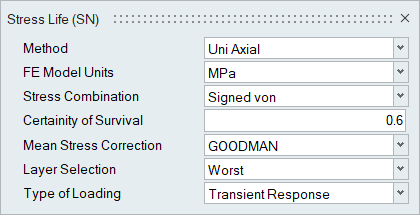
Figure 4.
Assign Materials
-
Click the Material tool.

Figure 5.The Assign Material dialog opens. -
Create a new material.
-
Click
 to create a new material.
-
Click Plot & Save.
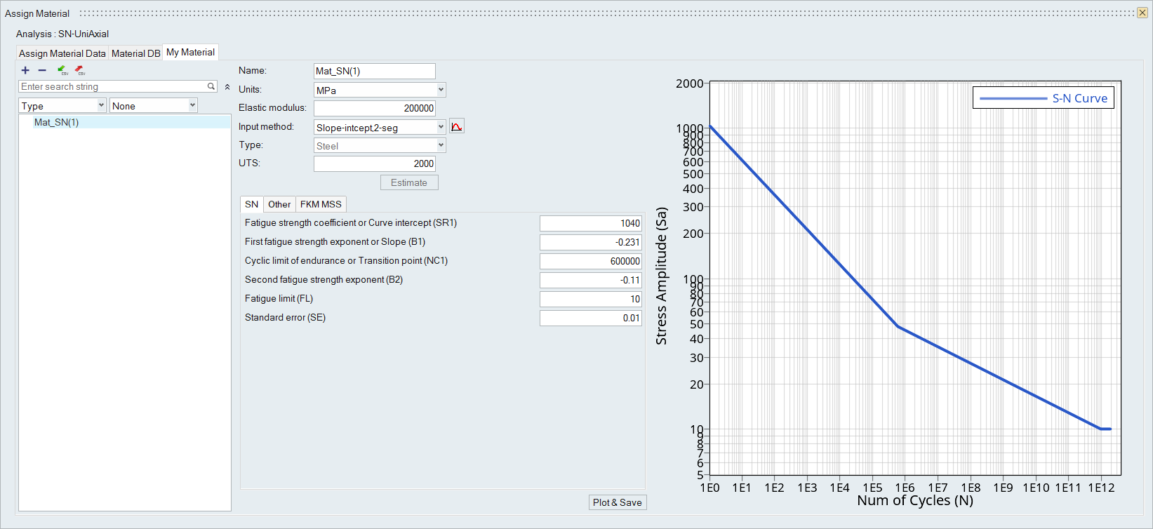
Figure 6.
-
Click
-
Click
 under Finish. In the
Surface Finish dialog, select
POLISH from the drop-down menu then click
OK.
under Finish. In the
Surface Finish dialog, select
POLISH from the drop-down menu then click
OK.
-
Click under Surf Treatment. In
the Surface Treatment dialog, select
NITRIDED from the drop-down menu then click
OK.
-
Set the Kf value to 1.3.
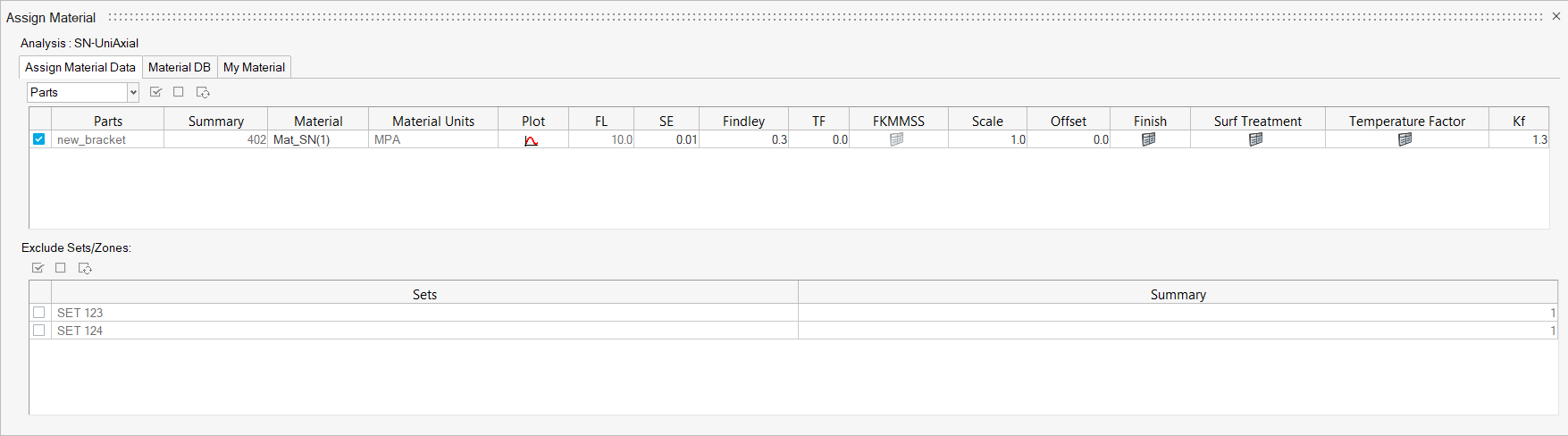
Figure 7.
Create a Transient Event
-
Click the Load Map tool.

Figure 8.The Load Map dialog opens.By default, the Channel Type is set to Transient Response and can not be changed. Since this is a transient fatigue analysis, a load history is not required.
-
On the bottom half of the dialog, click to create an Event_1 header.
Subcase 1 is listed under the event.
-
Activate the Event_1 checkbox.
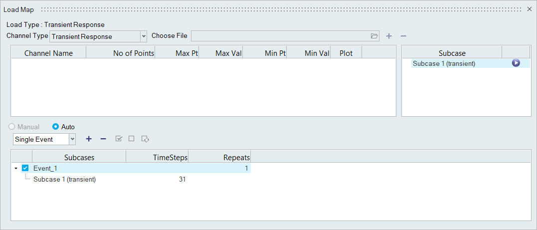
Figure 9.Note: You can only select one transient subcase per event.
Evaluate and View Results
-
From the Evaluate tool group, click the
Run Analysis tool.

Figure 10.The Evaluate dialog opens.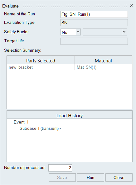
Figure 11. -
Use the Results Explorer to
visualize various types of results.
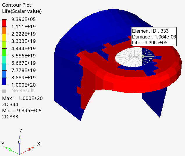
Figure 12.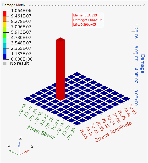
Figure 13.